Chapter 4

4.1 Introduction

In the rapidly evolving landscape of economics and social sciences, the advent of predictive models has heralded a new era of analysis and decision-making. These models, leveraging vast amounts of data and sophisticated algorithms, offer unprecedented insights into future trends, behaviors, and outcomes. From forecasting economic growth and market dynamics to predicting social phenomena and public health crises, predictive models have become indispensable tools for researchers, policymakers, and business leaders alike.

This chapter delves into the core concepts and methodologies underpinning predictive modeling, providing a comprehensive overview of both traditional statistical approaches and advanced machine learning techniques. We explore their theoretical foundations, practical applications, and the challenges encountered in real-world implementations. Special attention is given to models such as linear regression, time series analysis, machine learning algorithms like random forests and neural networks, and innovative approaches including natural language processing (NLP) and deep learning.

Moreover, we examine the profound impact of predictive models on economic policy formulation, social program design, and strategic business decisions. Through case studies and examples, we illustrate how these models inform evidence-based policymaking, optimize resource allocation, enhance market analysis, and contribute to solving complex economic and social issues.

By the end of this chapter, readers will gain a thorough understanding of the pivotal role of predictive models in economic and social research, equipped with the knowledge to apply these tools in diverse contexts and contribute to informed decision-making processes in the face of uncertainty.

4.2 Linear Regression Models Google Colab

Linear regression models serve as the cornerstone in the realms of economics and social sciences, facilitating the prediction of continuous outcomes from one or multiple predictor variables. Their widespread application spans forecasting pivotal economic indicators such as GDP growth, inflation rates, and employment levels, leveraging historical data and trends. This section elucidates the principles underlying linear regression, explores its application in economic forecasting, and discusses methodological considerations for ensuring robust model performance.

4.2.1 Simple Linear Regression

Simple linear regression involves fitting a linear model to the relationship between two variables: one independent variable $X$ and one dependent variable $Y$ . The model can be expressed as:

Y = β0 + β1X + 𝜖

where:

$Y$ is the dependent variable,
$X$ is the independent variable,
$β0$ is the intercept,
$β1$ is the slope coefficient,
$𝜖$ is the error term representing the difference between the observed and predicted values.

4.2.1.1 Example

Consider a simple example where we want to predict the annual salary ( $Y$ ) based on years of experience ( $X$ ). Suppose we have the following data:

Years of Experience (X) Salary ($) (Y ) 1 40,000 2 45,000 3 50,000 4 55,000 5 60,000

Using simple linear regression, we can fit the model:

ˆY = 35,000 + 5,000X

In this example, $β0 = 35,000$ and $β1 = 5,000$ . The intercept $β0$ represents the expected salary with zero years of experience, and $β1$ indicates the increase in salary for each additional year of experience.

4.2.2 Multiple Linear Regression

Multiple linear regression extends simple linear regression to include multiple independent variables. The model can be expressed as:

Y = β0 + β1X1 + β2X2 + ...+ βnXn + 𝜖

where:

$Y$ is the dependent variable,
$X1,X2, ...,Xn$ are the independent variables,
$β0,β1,...,βn$ are the coefficients,
$𝜖$ is the error term.

4.2.2.1 Example

Consider an example where we want to predict house prices ( $Y$ ) based on various factors such as the size of the house in square feet ( $X1$ ), the number of bedrooms ( $X2$ ), and the age of the house in years ( $X3$ ). Suppose we have the following data:

Size (sq ft) (X1) Bedrooms (X2 ) Age (years) (X3 ) Price ($) (Y ) 1500 3 10 300,000 1600 3 8 320,000 1700 4 5 340,000 1800 4 2 360,000 1900 5 1 380,000

Using multiple linear regression, we can fit the model:

ˆY = 200,000 + 100X1 + 20,000X2 − 1,000X3

In this example, $β0 = 200,000$ , $β1 = 100$ , $β2 = 20,000$ , and $β3 = − 1,000$ . The intercept $β0$ represents the baseline house price, $β1$ represents the price increase per square foot, $β2$ represents the price increase per additional bedroom, and $β3$ represents the price decrease per additional year of age.

4.2.3 Model Evaluation

To evaluate the performance of a linear regression model, we commonly use metrics such as the Mean Squared Error (MSE), Root Mean Squared Error (RMSE), and $R2$ (coefficient of determination). These metrics help to quantify the accuracy of the predictions and the goodness of fit of the model.

4.2.3.1 Mean Squared Error (MSE)

The Mean Squared Error is defined as:

n∑ MSE = 1- (Yi − ˆYi)2 n i=1

where $Yi$ is the actual value, $ˆYi$ is the predicted value, and $n$ is the number of observations.

4.2.3.2 Root Mean Squared Error (RMSE)

The Root Mean Squared Error is the square root of the MSE:

√----- RMSE = MSE

4.2.3.3 $R2$ (Coefficient of Determination)

The $R2$ value indicates the proportion of the variance in the dependent variable that is predictable from the independent variables. It is defined as:

∑n ˆ 2 R2 = 1− -∑in=1(Yi −-Yi) i=1(Yi − ¯Y)2

where $¯ Y$ is the mean of the observed values.

4.2.3.4 Example of Model Evaluation

Consider the simple linear regression example above where we predicted the annual salary based on years of experience. Suppose we have the following actual and predicted salaries:

Years of Experience (X ) Actual Salary ($) (Y) Predicted Salary ($) () 1 40,000 40,000 2 45,000 45,000 3 48,000 50,000 4 56,000 55,000 5 59,000 60,000

The MSE can be calculated as:

1[ 2 2 2 2 2] MSE = 5 (40,000 − 40,000) + (45,000− 45,000) + (48,000− 50,000) + (56,000− 55,000) + (59,000 − 60,000)

MSE = 1[0+ 0 +4,000 +1,000 +1,000] = 6,000 = 1,200 5 5

The RMSE is:

∘ ----- RMSE = 1,200 ≈ 34.64

The $R2$ value can be calculated as:

∑5 (Yi − ˆYi)2 R2 = 1− -∑i5=1-----¯-2 i=1(Yi − Y)

Assuming the mean salary $¯Y$ is 49,600, we have:

R²	= 1 −
	= 1 −
	= 1 −
	= 1 −
	≈ 0.92

This indicates that approximately 92% of the variance in salary is explained by years of experience.

4.2.4 Conclusion

Linear regression models are powerful tools for predicting continuous outcomes and understanding relationships between variables. By carefully selecting and evaluating models, economists and social scientists can derive meaningful insights and make informed predictions based on historical data.

4.3 Time Series Forecasting Models Google Colab

Time series forecasting involves predicting future values of a time series based on its historical data. This guide covers different approaches to time series forecasting and delves into various models, providing both beginners and advanced users with a thorough understanding.

4.3.1 Recursive Forecasting

In recursive forecasting, a model is trained on historical data, and predictions are made one step at a time. Each forecasted value is fed back into the model to predict the next time step.

Advantages: Simple implementation, works well for short-term predictions.
Disadvantages: Errors can accumulate over time, making long-term predictions less accurate.

Example: Suppose we have a time series of daily temperatures, T_t. We train a model on the historical data up to day t, and use it to predict the temperature on day t + 1, denoted as T_t+1. This predicted value T_t+1 is then used along with the historical data to predict the temperature on day t + 2, denoted as T_t+2, and so on.

4.3.2 Rolling Window Forecasting

In rolling window forecasting, the model is trained on a fixed window of the most recent historical data. This window rolls forward in time as predictions are made.

Advantages: Better adapts to changes in the time series, reduces the impact of old data.
Disadvantages: Requires more computational power, choosing the window size can be challenging.

Example: Assume we have a time series of stock prices, P_t, and we use a rolling window of size n. We train our model on the most recent n observations, {P_t−n+1,P_t−n+2,…,P_t}, to forecast the stock price on day t + 1, P_t+1. For the next prediction, the window rolls forward, and we use {P_t−n+2,P_t−n+3,…,P_t+1} to forecast P_t+2.

4.3.3 Stationarity

Stationarity is a property of a time series whereby its statistical properties, such as mean and variance, are constant over time. Stationarity is crucial for many time series models to perform accurately.

Example: Consider a time series of monthly sales data. If the mean and variance of the sales data remain roughly constant over different periods, the series can be considered stationary. However, if there are trends or seasonality, the series is non-stationary and needs to be transformed.

4.3.4 Tests for Stationarity

Common tests for stationarity include:

Augmented Dickey-Fuller (ADF) Test: A hypothesis test where the null hypothesis is that the series has a unit root (is non-stationary).
Kwiatkowski-Phillips-Schmidt-Shin (KPSS) Test: A hypothesis test where the null hypothesis is that the series is stationary.
Phillips-Perron (PP) Test: Another test for a unit root that is similar to the ADF test but makes different assumptions about the data.

Example: To check if a time series of quarterly GDP data is stationary, we can apply the ADF test. If the p-value is below a certain threshold (e.g., 0.05), we reject the null hypothesis and conclude that the series is stationary. Otherwise, we may need to difference the series to achieve stationarity.

4.3.5 Differencing

Differencing is a method used to transform a non-stationary time series into a stationary one by subtracting the previous observation from the current observation.

Yt = Xt − Xt−1

This process can be repeated (known as second differencing, third differencing, etc.) until the series becomes stationary. Differencing helps to remove trends and seasonality, making the time series suitable for modeling.

Example: Suppose we have a time series of monthly airline passengers, P_t, which shows an increasing trend. By applying first differencing, we obtain Y _t = P_t −P_t−1. If the series still exhibits non-stationarity, we might apply second differencing: Z_t = Y _t − Y _t−1. The differenced series can then be used to train models like ARIMA.

4.3.6 Types of Time Series Forecasting Models

4.3.6.1 Autoregression (AR)

Autoregression is a model that uses the dependency between an observation and a number of lagged observations (i.e., past values).

∑p Xt = c + ϕiXt− i + 𝜖t i=1

where X_t is the value at time t, c is a constant, ϕ_i are the coefficients, p is the number of lagged observations, and 𝜖_t is white noise.

Example: Suppose we have quarterly sales data for a company, S_t. An AR(2) model would use the previous two quarters’ sales to predict the current quarter’s sales:

St = c+ ϕ1St− 1 + ϕ2St−2 + 𝜖t

4.3.6.2 Moving Average (MA)

Moving average models use the dependency between an observation and a residual error from a moving average model applied to lagged observations.

∑q Xt = μ+ 𝜃i𝜖t−i + 𝜖t i=1

where X_t is the value at time t, μ is the mean of the series, 𝜃_i are the coefficients, q is the order of the model, and 𝜖_t is white noise.

Example: For monthly temperature data, T_t, an MA(1) model would use the previous month’s error term to predict the current month’s temperature:

Tt = μ+ 𝜃1𝜖t−1 + 𝜖t

4.3.6.3 Autoregressive Moving Average (ARMA)

ARMA combines AR and MA models to account for both lagged observations and lagged forecast errors.

∑p ∑q Xt = c+ ϕiXt−i + 𝜃j𝜖t− j + 𝜖t i=1 j=1

where p is the order of the autoregressive part and q is the order of the moving average part.

Example: Suppose we have a time series of daily water consumption, W_t. An ARMA(1,1) model would use both the previous day’s consumption and the previous day’s error term to predict the current day’s consumption:

Wt = c+ ϕ1Wt− 1 + 𝜃1𝜖t−1 + 𝜖t

4.3.6.4 Autoregressive Integrated Moving Average (ARIMA)

ARIMA models are an extension of ARMA that incorporate differencing to make the time series stationary.

∑p ∑q (1− ϕiLi)(1 − L)dXt = c +(1 + 𝜃jLj)𝜖t i=1 j=1

where L is the lag operator, d is the degree of differencing. The ARIMA model is characterized by three parameters:

p: The number of lag observations included in the model (lag order).
d: The number of times that the raw observations are differenced (degree of differencing).
q: The size of the moving average window (order of moving average).

Example: For a non-stationary time series of weekly website visits, W_t, we might first difference the series and then apply an ARIMA(1,1,1) model:

∇Wt = c+ ϕ1∇Wt −1 + 𝜃1𝜖t− 1 + 𝜖t

4.3.6.5 Autoregressive Distributed Lag (ARDL)

ARDL models are used when there are multiple time series, and the goal is to predict the value of one series using the lagged values of itself and other series.

∑p ∑q Yt = c+ ϕiYt−i + βjXt− j + 𝜖t i=1 j=0

where Y _t is the dependent variable, X_t is the independent variable, ϕ_i and β_j are coefficients, and p and q are the lag orders.

Example: Suppose we have monthly data on consumer spending (C_t) and income (I_t). An ARDL model might predict consumer spending based on its past values and past values of income:

∑p ∑q Ct = c+ ϕiCt−i + βjIt− j + 𝜖t i=1 j=0

4.3.6.6 Seasonal Decomposition of Time Series (STL)

STL is a method for decomposing a time series into seasonal, trend, and residual components.

Example: For a time series of daily electricity consumption, we can decompose the series as follows:

Yt = Tt + St + Rt

where T_t is the trend component, S_t is the seasonal component, and R_t is the residual component. This decomposition can help isolate seasonal effects and better understand underlying patterns.

4.3.6.7 Exponential Smoothing (ETS) Model

Exponential Smoothing models are a family of models that predict future values by averaging past observations with exponentially decreasing weights.

2 ˆYt+1 = αYt + α(1− α)Yt−1 + α(1− α) Yt−2 + ⋅⋅⋅

(1)

where α is the smoothing parameter.

Example: For a time series of monthly sales, S_t, an ETS model would use the exponentially weighted average of past sales data to predict the next month’s sales:

2 ˆSt+1 = αSt + α(1− α)St−1 + α(1− α )St−2 + ⋅⋅⋅

4.3.6.8 Vector Autoregression (VAR)

VAR models are used when there are multiple time series and we want to capture the linear interdependencies among them.

p Yt = c+ ∑ ΦiYt−i + 𝜖t i=1

where Y _t is a vector of time series variables, Φ_i are matrices of coefficients, and 𝜖_t is a vector of errors.

Example: Suppose we have monthly data on inflation (I_t) and unemployment (U_t). A VAR model would allow us to model the relationship between these two series simultaneously:

( ) ( )( ) It = c+ Φ11 Φ12 It−1 + 𝜖t Ut Φ21 Φ22 Ut− 1

4.3.7 Conclusion for Time Series Forecasting

Time series forecasting is a crucial tool in various domains, including finance, economics, and weather forecasting. By employing different approaches and models, practitioners can make informed predictions based on historical data. Whether it’s recursive forecasting, rolling window forecasting, or more advanced models like ARIMA, understanding the underlying principles is essential for accurate forecasting.

4.4 Prophet Forecasting Google Colab

Prophet is an open-source forecasting tool developed by Facebook for time series data. It is designed to be easy to use while providing accurate forecasts, making it suitable for both beginners and experts.

4.4.1 Model Components

Prophet decomposes a time series into three main components: trend, seasonality, and holidays. The model is defined as follows:

y(t) = g(t)+ s(t) + h(t)+ 𝜖t

where:

$g(t)$ represents the trend component,
$s(t)$ represents the seasonal component,
$h(t)$ represents the holiday component,
$𝜖t$ represents the error term (residuals).

4.4.2 Trend Component

The trend component $g(t)$ models non-periodic changes in the value of the time series. Prophet offers two types of trend models: a piecewise linear model and a logistic growth model.

4.4.2.1 Piecewise Linear Trend

The piecewise linear trend allows the growth rate to change at specified points in time, known as change points. This is useful for time series data that exhibit different growth rates during different periods.

For example, consider a company’s revenue that experiences different growth rates before and after a major product launch. The piecewise linear trend can model such changes in growth rates effectively.

The piecewise linear trend is defined as:

T T g(t) = (k + a(t) δ)t+ (m +a(t) γ)

where:

$k$ is the growth rate,
$m$ is the offset parameter,
$a(t)$ is a vector of change points indicators,
$δ$ and $γ$ are the adjustments to the rate and offset at the change points.

4.4.2.2 Logistic Growth Trend

The logistic growth model is suitable for time series that saturate at a certain carrying capacity $C$ . This is useful in scenarios where the growth is initially exponential but slows down as it approaches a saturation point.

For instance, the adoption of a new technology often follows a logistic growth curve: rapid initial adoption that slows as the market becomes saturated.

The logistic growth trend is defined as:

g(t) =--------C-------- 1 + exp(− k(t− t0))

where:

$C$ is the carrying capacity,
$k$ is the growth rate,
$t0$ is the time at which the growth rate is maximum.

4.4.3 Seasonality Component

The seasonal component $s(t)$ captures periodic changes in the time series. Prophet uses Fourier series to model seasonality, which allows it to handle multiple seasonal patterns simultaneously.

For example, a retail business might experience daily, weekly, and yearly seasonal patterns. Daily patterns could reflect customer behavior during different times of the day, weekly patterns might show differences between weekdays and weekends, and yearly patterns could account for holiday effects and other annual events.

The seasonality is modeled as:

N [ ( ) ( ) ] s(t) = ∑ ancos 2πnt +bn sin 2πnt n=1 P P

where:

$N$ is the number of Fourier terms,
$an$ and $bn$ are the coefficients,
$P$ is the period of the seasonality (e.g., 365.25 for yearly seasonality).

4.4.4 Holiday Component

The holiday component $h (t)$ allows for the inclusion of user-specified holidays and special events. This is particularly useful for businesses that experience significant variations in activity during holidays or special events.

For instance, retail sales might spike during Black Friday or Christmas. By including these holidays in the model, Prophet can account for their impact on the time series.

The holiday effect is modeled as:

∑ ( ) h(t) = 1holiday(t,k) ⋅βk k

where $βk$ is the parameter representing the effect of holiday $k$ .

4.4.5 Error Term

The error term $𝜖t$ represents the residuals or noise in the data. Prophet assumes the residuals to be normally distributed:

2 𝜖t ∼ 𝒩 (0,σ )

4.4.6 Model Fitting

Prophet uses maximum likelihood estimation to fit the model parameters. The fitting process involves:

Identifying change points in the trend,
Estimating the Fourier series coefficients for seasonality,
Incorporating holiday effects,
Optimizing the parameters using an iterative algorithm.

4.4.7 Forecasting with Prophet

To make forecasts with Prophet, follow these steps:

Prepare the Historical Data: Organize your historical time series data with columns for the date (ds) and the value (y). Specify any holidays or special events that should be included in the model.
Fit the Prophet Model: Apply the Prophet model to your historical data to estimate the trend, seasonality, and holiday effects.
Make Predictions: Use the fitted model to generate future forecasts.

4.4.8 Example: Forecasting Retail Sales

Consider a retail business that wants to forecast its daily sales. The data includes daily sales figures for the past three years, and the company experiences significant sales increases during Black Friday and Christmas.

4.4.9 Step 1: Prepare the Data

The historical sales data is organized with columns for the date and sales. Holidays such as Black Friday and Christmas are specified.

4.4.10 Step 2: Fit the Model

The Prophet model is applied to the historical data, accounting for trend changes, yearly seasonality, and the specified holidays.

4.4.11 Step 3: Make Predictions

Using the fitted model, the company generates a forecast for the next year. The forecast includes the expected sales increase during Black Friday and Christmas, as well as the overall trend and seasonality patterns.

4.4.12 Conclusion

Prophet offers a powerful yet user-friendly approach to time series forecasting. Its ability to decompose time series into trend, seasonality, and holiday components simplifies the forecasting process. With Prophet, even beginners can generate accurate forecasts for their time series data. By leveraging Prophet’s capabilities, forecasters can make informed decisions and anticipate future trends with confidence.

4.5 Neural Networks and Deep Learning

Neural networks and deep learning models excel in processing large, complex datasets to uncover patterns that may elude simpler models or human analysis. This subsection covers their application in economic forecasting, sentiment analysis of social media, and fraud detection in financial transactions, emphasizing their structure, functionality, and the pivotal role of data in model training and validation.

4.5.1 Introduction to Neural Networks and Deep Learning

Neural networks represent a cornerstone of modern computational intelligence, driving advancements in various domains by processing large and complex datasets with unparalleled efficiency. This section introduces the fundamental concepts underlying neural networks and deep learning, aiming to elucidate their structure, functionality, and broad applications.

Objective: The primary goal is to equip readers with a basic understanding of neural networks and their significance in analyzing vast datasets. This understanding is crucial for leveraging deep learning technologies in practical applications, from economic forecasting to security enhancements in financial transactions.
Processing Large, Complex Datasets: At the heart of neural networks’ transformative power is their capability to sift through, analyze, and extract meaningful patterns from datasets that are too large and complex for traditional statistical methods. This attribute has made neural networks a go-to solution for handling the ever-increasing volume of data in various fields.
Applications: Neural networks have found applications across a diverse set of fields, demonstrating their versatility and effectiveness:
- Economic forecasting: By analyzing historical and current economic data, neural networks improve the accuracy of predictions concerning economic trends, benefiting policymakers and investors alike.
- Sentiment analysis: The ability to analyze vast amounts of unstructured data from social media and news outlets allows neural networks to gauge market sentiment, providing valuable insights into consumer behavior and market trends.
- Fraud detection: Neural networks enhance the security of financial transactions by effectively identifying patterns indicative of fraudulent activities, thereby protecting individuals and institutions from financial losses.
Structure and Functionality: An overview of the architecture of neural networks lays the foundation for understanding their functionality. This section delves into how neural networks are constructed, including the interconnections between nodes (neurons) and layers, and how these structures enable the processing of complex data inputs to generate actionable insights.

In conclusion, the advent of neural networks and deep learning technologies marks a significant milestone in the evolution of computational methods, offering powerful tools for data analysis and decision-making in economic and financial analysis, among other areas.

4.5.2 What are Neural Networks?

Neural networks constitute a pivotal model in predictive analytics, enabling the forecasting of outcomes through sophisticated analysis of input variables. This section unpacks the essence of neural networks, highlighting their primary components and the roles these components play in predictive modeling.

At its core, a neural network is a computational model designed to predict outcomes by processing a set of input variables. This predictive capability is foundational to its application across various scientific, economic, and technological domains.
Components: The functionality of neural networks is attributed to several key components, each contributing to the network’s ability to model complex relationships:
- Input vector $(X1, X2,...,Xn )$ : Represents the set of input variables fed into the neural network. These inputs are the starting point from which the network begins its analysis and prediction process.
- Nonlinear function $f(X )$ : At the heart of a neural network’s predictive power is a nonlinear function that maps the input variables to the output. This function is capable of capturing the intricate and complex relationships between the inputs and the resulting output, a feature that linear models lack.
- Predictive modeling of response $Y$ : The ultimate goal of the neural network is to model the response or outcome $Y$ based on the input variables $X$ . This involves learning from data to understand how changes in the input variables are likely to affect the outcome, thereby enabling accurate predictions.

By dissecting the components and operational mechanics of neural networks, this section aims to provide readers with a clear understanding of how these powerful models function. Through the interplay of input vectors, nonlinear functions, and predictive modeling, neural networks offer a robust framework for tackling complex prediction tasks across myriad applications.

4.5.3 Structure of a Neural Network

The architecture of a neural network is a defining aspect that enables it to perform complex computations and model relationships within data. This section details the essential layers that make up a neural network and the roles they play in processing information.

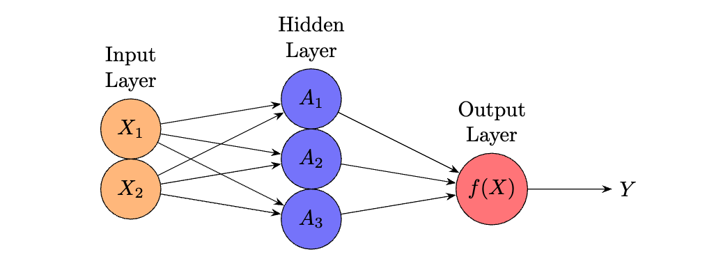
Figure 1: A simple feed-forward neural network for modeling a quantitative response using 2 predictors and 3 hidden units.

The structure of a neural network can be conceptualized as comprising several distinct layers, each with a specific function:

Input Layer: This layer serves as the entry point for the input signals $(X1, X2,...,Xn )$ . It’s responsible for receiving the input features and passing them on to the next layer for further processing.
Hidden Layer(s): Positioned between the input and output layers, hidden layers are crucial for the neural network’s ability to capture complex relationships in the data. They process inputs through weighted connections and employ nonlinear activation functions to enable the network to learn and model non-linearities.
Output Layer: The final layer in the neural network architecture, the output layer produces the network’s output. This output can vary depending on the specific task the network is designed for, such as generating a continuous value for regression tasks or a class label for classification tasks.
Formulae: The operational dynamics of a neural network are determined by the interconnectedness of these layers, the weights assigned to each connection, and the choice of activation functions. These weights are fine-tuned during the training process to minimize the difference between the predicted output and the actual target values.

The structure outlined here provides a foundation for understanding how neural networks manage to perform a wide range of tasks, from simple pattern recognition to complex decision-making processes. By adjusting the weights and biases through training, neural networks learn to approximate the function that maps inputs to outputs, thus becoming increasingly proficient at predicting outcomes based on unseen input data.

4.5.4 Mathematical Formulation of a Neural Network

A neural network models the relationship between inputs and outputs through a series of mathematical operations, defined by a structured network of nodes or neurons. The mathematical formulation of a neural network provides a framework for understanding how inputs are transformed into outputs, emphasizing the role of parameters that are adjusted during the learning process.

The general form of a neural network model can be expressed as follows:

f(X)	= β₀ + ∑ _k=1³β_kh_k(X)	(1)
	= β₀ + ∑ _k=1³β_kg	(2)

This formulation encapsulates the process of constructing a neural network model in two primary steps:

The model begins by computing the activations $Ak$ for $k = 1,...,3$ , within the hidden layer. These activations are functions of the input features $X1,X2$ , calculated as:

$( 2 ) A = h (X ) = g(w + ∑ w X ) k k k0 j=1 kj j$ (3)

Here, $g$ denotes a nonlinear activation function, a crucial component that allows the neural network to capture complex, non-linear relationships between the inputs and outputs. The choice of $g$ significantly influences the network’s performance and its ability to model complex patterns.
The next step involves estimating the model parameters, which include $β0,β1,β2,β3$ for the output layer and $w10,w11,w12,w20,w21,w22,w30,w31,w32$ for the activations in the hidden layer. These parameters are optimized through a process that typically involves minimizing a loss function that quantifies the difference between the predicted outputs and the actual data. This optimization is achieved using algorithms such as gradient descent, which iteratively adjusts the parameters to improve the model’s predictions.

Through this mathematical framework, a neural network learns to approximate the function that maps inputs to outputs, adjusting its parameters based on the data it is trained on. The structure and optimization of these parameters are key to the network’s ability to learn and make accurate predictions.

4.5.5 Activation Functions in Neural Networks

Activation functions are the heartbeat of neural networks, injecting the necessary non-linearity to model complex data patterns. This segment explores the quintessential roles of two cornerstone activation functions: the Sigmoid and Rectified Linear Unit (ReLU), highlighting their distinct attributes and contributions to neural network architectures.

Historical and Modern Preferences:

The Sigmoid function has played a foundational role in neural network evolution. By elegantly mapping input values to a (0, 1) range, it facilitated early networks’ ability to interpret outputs as probabilities, making it particularly valuable for classification tasks.
The ReLU function marks a shift towards modernity, prized for its computational efficiency and its strategic mitigation of the vanishing gradient issue, a common obstacle in the training of deep networks.

Functional Insights: Sigmoid Function: $1 g(z) = 1+e−z$ , a hallmark in logistic regression, is adept at transforming inputs to probability spaces, proving indispensable in binary classification scenarios.

ReLU Function: $g(z) = max (0,z)$ , stands out for its operational simplicity, fostering faster learning by directly passing positive inputs while nullifying negatives, a property that accelerates network training.

Visualization and Impact:

Figure 2: Contrasting dynamics of Sigmoid and ReLU activation functions, highlighting the Sigmoid’s smooth transition against ReLU’s piecewise linearity.

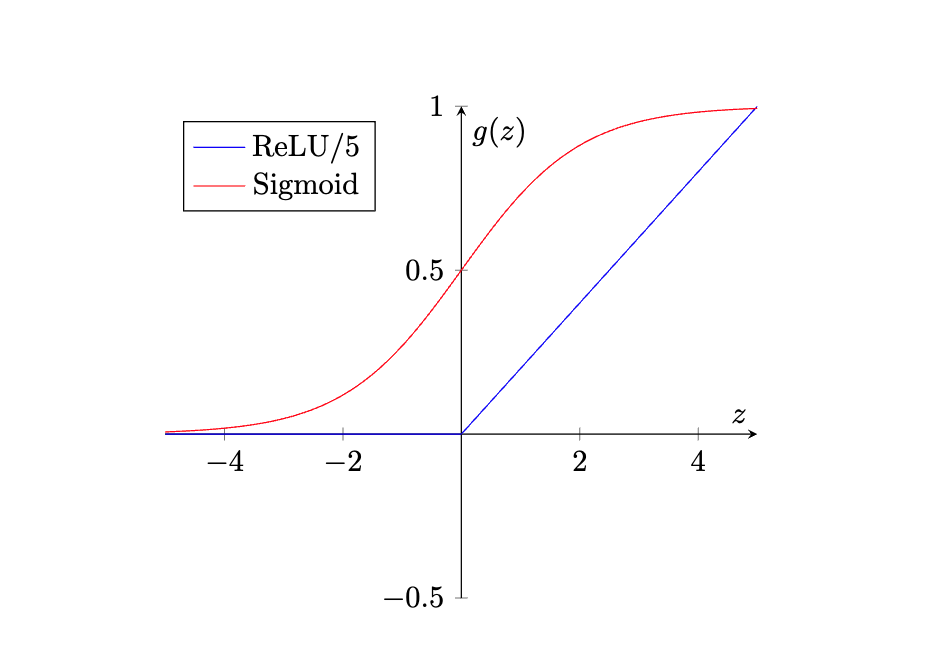
The transition from Sigmoid to ReLU encapsulates a broader narrative of innovation within neural network research, underscoring a relentless pursuit of more efficient, capable models. The choice between these functions is not merely technical but strategic, profoundly influencing a network’s learning efficiency and problem-solving capacity.

In sum, the evolution from Sigmoid to ReLU is emblematic of neural networks’ journey towards achieving higher levels of complexity and functionality. This choice of activation function, far from being a mere detail, plays a critical role in defining a network’s architecture, its training behavior, and ultimately, its success in application.

4.5.6 Understanding Parameter Estimation in Neural Networks

Parameter estimation is a fundamental aspect of training neural networks, underpinning the model’s ability to learn from data and make accurate predictions. This section delves into the core components of parameter estimation: the squared-error loss function and the optimization process, each playing a pivotal role in refining the model’s parameters.

Squared-Error Loss Function: At the heart of regression tasks within neural networks lies the squared-error loss function. This function quantifies the difference between the predicted outputs of the network and the actual target values. Its primary objective is to minimize the sum of the squared differences, providing a measure of the model’s prediction accuracy.

Objective: The squared-error loss function aims to minimize the discrepancy between the network’s predictions ( $f(xi)$ ) and the actual observations ( $yi$ ), thus improving the model’s predictive performance.
Formula: The loss is calculated as $∑ 2 L = (yi − f (xi))$ , representing the cumulative squared difference across all data points.

Optimization Process: Optimization is the iterative process through which the model’s parameters ( $β$ , $w$ ) are adjusted to reduce the loss function. This process is crucial for fine-tuning the network’s weights, steering the model towards higher accuracy and reliability.

Figure 3: Illustration of the Optimization Process via Gradient Descent, highlighting the methodical adjustment of parameters to minimize the loss function.

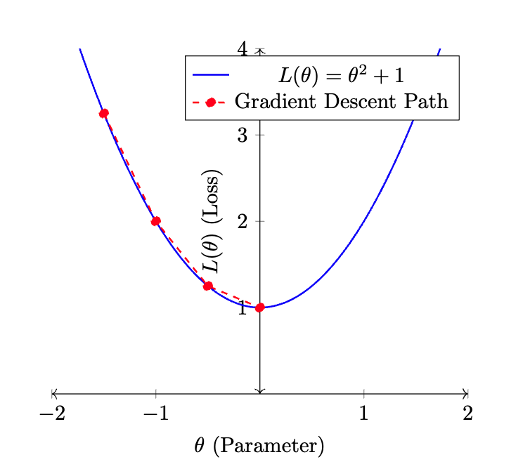
Methods: Techniques such as Gradient Descent are employed to navigate the parameter space, seeking configurations that minimize the loss. These methods iteratively update the model’s weights based on the gradient of the loss function, effectively reducing prediction error over time.
Adjustments: Through incremental adjustments, the optimization process ensures that the model’s parameters are refined, aligning the predicted outputs more closely with the actual target values.

Parameter estimation, encapsulating both the formulation of the loss function and the iterative optimization of model parameters, is indispensable for the development of effective neural networks. Through this rigorous process, models are equipped to capture the underlying patterns in data, enhancing their predictive accuracy and utility in real-world applications.

4.5.7 Fitting Neural Networks

The task of fitting neural networks is a blend of complexity and sophistication, requiring a balance between theoretical understanding and practical application. It is an inherently adaptive process, characterized by iterative optimization and fine-tuning of the network’s parameters to best capture the underlying patterns within the data. This complexity arises from the need to navigate a vast parameter space, adjust for overfitting, and ensure that the model generalizes well to unseen data.

Complexity in Fitting: Fitting neural networks involves a deep engagement with both the architecture of the model and the characteristics of the dataset. It’s a task that demands not only computational resources but also a nuanced understanding of how different model configurations might perform under various conditions. This complexity is not just a barrier; it represents the rich potential of neural networks to model an extensive range of phenomena across different domains.

Easing the Process with Software: Thankfully, the advancement of computational tools and software has significantly demystified the process of fitting neural networks. Modern software packages provide comprehensive frameworks that abstract much of the complexity involved in neural network design and training. These tools offer intuitive interfaces and automated processes for tasks such as parameter tuning, model evaluation, and deployment, making neural networks more accessible to practitioners across fields. This accessibility is crucial for harnessing the power of neural networks in solving real-world problems, from image recognition to natural language processing and beyond.

Key Takeaway: The main takeaway is that, despite the inherent challenges in understanding and fitting neural networks, the availability of advanced computational tools has greatly facilitated this process. These tools bridge the gap between theoretical complexity and practical applicability, allowing users to effectively leverage neural networks with a fraction of the effort once required. As these technologies continue to evolve, we can anticipate even greater ease of use, enabling broader adoption and innovation in the application of neural networks.

In conclusion, the journey from conceptualizing to effectively fitting neural networks encapsulates the dynamic interplay between theoretical depth and practical tooling. While the complexity of the task underscores the sophisticated nature of these models, the development of user-friendly software tools signifies a pivotal shift towards making powerful neural network technologies accessible to a wider audience.

4.5.8 Empowering Economics and Finance with Neural Networks

Neural networks, as a pivotal advancement in artificial intelligence, have ushered in a new era of economic forecasting and financial analysis. By harnessing their pattern recognition and predictive capabilities, these models offer unprecedented insights into complex market dynamics and decision-making processes.

Recap on Importance: Neural networks stand at the forefront of the intersection between technology and financial analysis, enabling a level of nuance and precision previously unattainable. Their adoption across economic and financial applications reflects a broad recognition of their potential to transform traditional practices:

By facilitating enhanced analysis of economic trends, neural networks empower policymakers and investors with more accurate forecasting tools, thereby improving the basis for critical decisions.
In the realm of finance, these AI models sift through vast datasets to unearth investment insights, thereby redefining strategies for market engagement and risk management.

Transformative Impact in Economics and Finance: The integration of neural network technology into economic and financial systems has marked a paradigm shift, with significant implications for forecasting, analysis, and risk management:

Economic Forecasting: The application of neural networks in predicting economic indicators exemplifies their value in enhancing the reliability of forecasts used by policymakers and market participants.
Financial Market Analysis: Leveraging vast amounts of data, AI models offer a deeper understanding of market trends, aiding in the identification of investment opportunities and the assessment of potential risks.
Risk Management: Through advanced algorithms, neural networks contribute to the detection of fraudulent activities and the evaluation of credit risk, significantly bolstering the security and efficiency of financial operations.

Looking Ahead: The trajectory of economic and financial sectors is increasingly aligned with the evolution of neural network technologies. As these models advance, their capacity to provide deeper insights and foster innovation within financial systems is set to expand, signaling a future where AI-driven analysis becomes a cornerstone of economic and financial strategy.

In summary, the intersection of neural networks with economics and finance not only illustrates the current impact of AI technologies but also highlights the immense potential for future advancements. As we look forward, the continued integration of neural networks promises to unlock new horizons in financial analysis, risk management, and economic forecasting, shaping the future of these fields.

4.6 Recurrent Neural Networks Google Colab

4.6.1 Recurrent Neural Networks: Overview and Applications

Recurrent Neural Networks (RNNs) represent a sophisticated class of neural networks, uniquely designed to handle sequential data. Unlike their feedforward counterparts, RNNs possess the remarkable ability to retain information across inputs, making them exceptionally adept at modeling time-dependent data. This characteristic enables RNNs to draw on past inputs to inform future predictions, essentially embodying a form of memory within the network’s architecture.

What are RNNs? RNNs are distinguished by their ability to process sequences of data, such as time series, speech, text, or any sequential observations. At the core of their design is the use of loops within the network, allowing information to be carried forward through each step of the input sequence. This design principle enables RNNs to maintain a dynamic state that evolves based on both new and historically processed information, facilitating the modeling of complex temporal behaviors.

Key Applications: In the realm of finance, RNNs have emerged as a powerful tool for analyzing time series data. They are extensively applied in predicting market trends, stock prices, and assessing financial risks. By leveraging historical market data, RNNs can forecast future values with a degree of accuracy unattainable by traditional statistical models. This predictive capability is invaluable for investors, analysts, and policymakers aiming to make informed decisions in the dynamic financial landscape.

Technical Insight: The operational backbone of RNNs lies in their sequential processing of information, characterized by the use of shared weights across temporal steps. This structure is inherently suited for financial applications such as tracking stock market indices and trading volumes, where the temporal dimension of data plays a critical role in prediction and analysis.

Practical Use: Advancements in computational software have significantly democratized access to RNN technologies, enabling financial analysts to employ these models without necessitating a granular understanding of their technical intricacies. Modern software platforms offer user-friendly interfaces and tools designed to streamline the development and deployment of RNNs for financial analysis, making sophisticated time series modeling more accessible than ever.

In conclusion, Recurrent Neural Networks have carved a niche in the financial sector, offering unparalleled insights into temporal data analysis. Through their unique architecture and the support of advanced software tools, RNNs have become an indispensable asset for financial time series analysis, predictive modeling, and risk assessment, underscoring their broad applicability and potential within the field.

4.6.2 The Structure of Simple Recurrent Neural Networks

Recurrent Neural Networks (RNNs) uniquely process sequential data, making them indispensable for capturing temporal dynamics. Unlike other neural network architectures, RNNs have the distinct capability to sequentially pass information across layers, thus retaining a memory of past inputs to inform future predictions. This ability is crucial for applications that rely on historical data to predict future events.

Temporal Dynamics and Memory: At the heart of RNNs is their ability to maintain a dynamic state, or "memory," of previous inputs. This memory is updated with each step in the input sequence, enabling the RNN to leverage accumulated historical information for making predictions. Such a feature renders RNNs particularly effective for tasks requiring an understanding of temporal sequences, such as time series forecasting, speech recognition, and natural language processing.

Operational Mechanism: Simplistically, an RNN takes an input sequence $X = {X ,X ,...,X } ℓ 1 2 L$ and produces a sequence of outputs. Each input $X ℓ$ at time step $ℓ$ influences the network’s hidden layer, updating its activations $A ℓ$ . These activations then inform the output at each step $O ℓ$ , leading to the final output $O L$ , which is reflective of the entire input sequence’s processed information.

Figure 4: Schematic of a simple recurrent neural network. The input sequence $L {Xℓ}1$ feeds sequentially into the hidden layer, which incorporates both the current input $Xℓ$ and the activation $A ℓ− 1$ from the previous sequence element to produce the current activation $A ℓ$ . The network employs consistent weights $W$ , $U$ , and $B$ throughout the sequence processing. 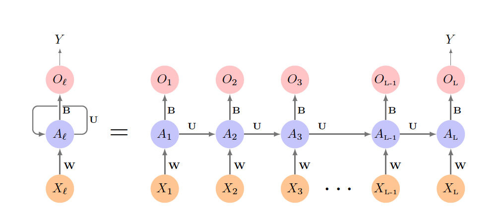While the output layer yields a sequence of predictions ${Oℓ}$ , typically only the final output $OL$ is utilized for response prediction. The diagram left of the equals sign compactly represents the network, which is expanded on the right for clarity.

L
{Xℓ}1 — Figure 4: Schematic of a simple recurrent neural network. The input sequence $L {Xℓ}1$ feeds sequentially into the hidden layer, which incorporates both the current input $Xℓ$ and the activation $A ℓ− 1$ from the previous sequence element to produce the current activation $A ℓ$ . The network employs consistent weights $W$ , $U$ , and $B$ throughout the sequence processing. While the output layer yields a sequence of predictions ${Oℓ}$ , typically only the final output $OL$ is utilized for response prediction. The diagram left of the equals sign compactly represents the network, which is expanded on the right for clarity.

Figure Overview: The figure provides a visual illustration of a simple RNN’s operational flow. It depicts how the network processes an input sequence by sequentially updating the hidden layer’s activations based on both the current input and the past activation state. This mechanism allows the network to synthesize and utilize the full spectrum of information contained within the sequence, culminating in a predictive output that reflects the integrated analysis of temporal data.

In essence, the structure of simple RNNs offers a potent framework for analyzing sequential data. By dissecting the operational principles of RNNs, we illuminate their vast applicability and potential in domains requiring nuanced temporal data analysis. The graphical representation further enhances comprehension of how these networks achieve their remarkable functionality, providing a solid foundation for understanding the interplay between sequential data processing and predictive modeling in RNNs.

4.6.3 RNN Mathematical Framework

Recurrent Neural Networks (RNNs) offer a dynamic architecture designed specifically for sequential data processing. Central to their operation is the ability to maintain a form of memory across inputs, enabling these networks to perform tasks that require an understanding of sequence context and temporal dependencies.

Overview of RNN Structure: RNNs distinguish themselves through a unique structure tailored to sequential input handling. This capability is rooted in their hidden layers, where information from past inputs is retained and utilized to inform predictions on future data points, making RNNs exceptionally suited for sequential tasks.

Input Vector $X ℓ$ : Each input vector $X ℓ$ in the sequence is composed of $p$ components, denoted as $X ⊤ = (X ,X ,...,X ) ℓ ℓ1 ℓ2 ℓp$ . This representation allows the network to handle complex data structures across different time steps effectively.

Hidden Layer Configuration: At every sequence step $ℓ$ , the hidden layer is comprised of $K$ units, represented by $⊤ A ℓ = (A ℓ1,Aℓ2,...,A ℓK )$ . These units are pivotal in capturing and propagating the temporal information throughout the network.

Weight Matrices and Vector:

Input Layer Weights ( $W$ ): A matrix of dimensions $K × (p + 1)$ , $W$ encapsulates the weights $wkj$ for the input layer, facilitating the transformation of input data into meaningful representations within the network.
Hidden-to-Hidden Weights ( $U$ ): The matrix $U$ of dimensions $K × K$ contains the weights $uks$ that govern the transitions between hidden states, enabling the network to integrate information over time.
Output Layer Weights ( $B$ ): A vector of length $K + 1$ , $B$ comprises the weights $βk$ for the output layer, which are instrumental in generating the final output from the network’s accumulated knowledge.

Hidden Layer Activation ( $A ℓk$ ): The activation of unit $k$ in the hidden layer at step $ℓ$ is given by:

( p K ) A = g (w + ∑ w X + ∑ u A ) ℓk k0 j=1 kj ℓj s=1 ks ℓ−1,s

where $g(⋅)$ represents a non-linear activation function, such as the ReLU, introducing the necessary non-linearity to model complex patterns in the data.

Output Computation ( $O ℓ$ ): The output at each step $ℓ$ is computed as:

K O ℓ = β0 + ∑ βkA ℓk k=1

This formulation allows for the generation of quantitative responses directly, or through additional functions like the sigmoid for binary outcomes, showcasing the versatility of RNNs.

Weight Sharing in RNNs: A key feature of RNNs is the sharing of weight matrices $W$ , $U$ , and vector $B$ across all steps of the sequence. This uniform application of learned transformations ensures that the network can generalize across different parts of the input sequence effectively.

Context Accumulation: As the network processes the input sequence, the hidden layer activations $A$ accumulate contextual information from previous steps. This accumulation allows the RNN to make informed predictions based on both the current input and the historical sequence context, highlighting the network’s capacity for temporal data integration and analysis.

The mathematical framework of RNNs elucidates the principles underpinning their design and functionality, providing a foundation for their application in a wide range of sequential data processing tasks. Through this framework, RNNs demonstrate a remarkable ability to model and predict complex patterns in temporal data, underscoring their significance in advancing the field of sequential data analysis.

4.6.4 Loss Function in RNNs for Regression Problems

Regression problems utilizing Recurrent Neural Networks (RNNs) concentrate on predicting continuous outcomes from sequential input data. The design and training of these models hinge significantly on the selection and implementation of an appropriate loss function, which quantifies the difference between the model’s predictions and the actual observed values.

Context of Regression in RNNs: In regression settings, RNNs aim to model and predict continuous variables by capturing the temporal dynamics inherent in sequential data. This predictive capability is pivotal for tasks where the outcome is a continuous measure influenced by preceding sequential inputs.

Loss Function Overview: The cornerstone of training RNN models for regression lies in the loss function. It serves as a measure of the model’s performance, indicating the extent of discrepancy between the predicted values by the network and the actual outcomes.

Definition of Loss Function: For a given observation pair $(X,Y )$ , with $X$ representing the sequential input and $Y$ the actual continuous value, the loss function in the context of RNNs for regression problems is typically defined as:

(Y − OL)2,

where $∑ OL = β0 + Kk=1βkALk$ denotes the final output of the RNN. This squared difference highlights the gap between the network’s prediction and the true value, guiding the model’s training process by minimizing this discrepancy.

Role of Intermediate Outputs: In the loss calculation, the emphasis is placed on the final output $OL$ , as it encapsulates the cumulative prediction based on the entire input sequence. The intermediate outputs, while crucial for arriving at $OL$ , do not directly influence the loss function.

Impact on Parameter Learning: The training of RNNs involves adjusting the shared parameters $W$ , $U$ , and $B$ , driven by the objective to minimize the loss function. Each element of the input sequence contributes to the final output through a series of transformations, underscoring the iterative learning process of these parameters to enhance prediction accuracy.

Importance in Model Fitting: Optimizing the shared parameters to reduce the loss is central to fitting RNN models for regression tasks. This optimization ensures that the model learns the intricate relationships between sequential inputs and their corresponding continuous outcomes, aiming for precise predictions.

Key Takeaway: The dynamics of the loss function are fundamental to the effective training of RNNs on sequential data for regression problems. Understanding and minimizing this loss is crucial for developing models that can accurately predict continuous values, reflecting the critical interplay between model architecture, parameter learning, and the objective measurement of prediction accuracy.

4.6.5 Application of RNNs in Financial Time Series Forecasting

Recurrent Neural Networks (RNNs) have emerged as a formidable tool in the domain of finance, particularly for the task of forecasting financial time series. Their intrinsic ability to process sequential data and capture temporal dependencies positions RNNs as a pivotal technology for modeling the often volatile and dynamic financial markets.

Introduction to RNNs in Finance: RNNs are adept at modeling the nuanced temporal patterns present in financial markets, making them highly effective for forecasting future market behaviors based on historical data. This capability is fundamental to understanding and anticipating market movements, offering valuable insights for investment and trading strategies.

Forecasting Objective: The primary goal in financial time series forecasting with RNNs is to predict future returns, such as the Dow Jones Industrial Average (DJ_return) at a subsequent time point $t$ . This objective leverages the sequential data processing strengths of RNNs, utilizing past market information to forecast future outcomes.

Data Structure and Preparation: To train RNN models, data is structured into mini-series of input sequences $X = {X1,X2,...,XL }$ , each with a specific lag $L$ . These sequences incorporate daily financial indicators—DJ_return ( $r$ ), log_volume ( $v$ ), and log_volatility ( $z$ )—capturing the market’s dynamics up to the point of interest.

Input Sequence Example: The formation of input sequences is illustrated as follows, where each $X ℓ$ represents a vector of financial indicators from day $t− L$ to $t− 1$ , aiming to predict the return $rt$ :

( ) ( ) ( ) rt−L rt−L+1 rt−1 X1 = ( vt−L) ,X2 = ( vt− L+1) ,...,XL = ( vt−1) , and Y = rt. zt−L zt− L+1 zt−1

Generating Training Data: Training datasets are constructed by creating $(X, Y)$ pairs for each value of $t$ from $L +1$ to $T$ , effectively forming a comprehensive dataset that mirrors the historical interplay among returns, volumes, and volatilities.

RNNs in Action: Through the analysis of these sequential datasets, RNNs endeavor to forecast future returns ( $rt$ ), drawing on learned patterns and dependencies across the various financial indicators to make informed predictions.

Significance: The deployment of RNNs in financial time series forecasting underscores their adaptability and efficacy in tackling complex forecasting tasks. This application highlights the potential of RNNs to enhance market return predictions using historical data, demonstrating their critical role in financial analysis and decision-making processes.

Note: The use of RNNs for predicting financial returns exemplifies their advanced capabilities in handling sequential data, providing profound implications for financial analysis and market prediction strategies. This showcases the transformative potential of RNNs in navigating the complexities of financial markets, offering a glimpse into the future of financial forecasting.

This subsection delves into the specifics of employing RNNs for financial time series forecasting, illustrating the model’s preparation, training, and predictive capabilities in the context of financial markets. It aims to convey the significance of RNNs in financial forecasting, demonstrating their utility in extracting meaningful insights from complex sequential data for predictive analysis.

4.7 Long Short-Term Memory (LSTM) Networks Google Colab

4.7.1 Overview of LSTM

LSTM networks, a specialized form of Recurrent Neural Network (RNN), are proficient in modeling sequence data, particularly for forecasting time series with long-term dependencies. This section addresses their theoretical underpinnings, distinguishes them from other RNN, and illustrates their application in predicting stock prices, currency exchange rates, and analyzing economic time series data, underscoring their significance in capturing temporal dynamics.

Overview of RNN and their limitations: Recurrent Neural Network (RNN) are uniquely suited for processing sequential data, as they maintain internal states that capture information from previous inputs. However, RNN face significant challenges in learning long-range dependencies due to vanishing and exploding gradients, making it difficult for earlier inputs to influence later outputs.

Introduction to LSTM: Long Short-Term Memory networks (LSTM) were introduced by Hochreiter & Schmidhuber in 1997 as an advanced RNN architecture designed to circumvent the problem of long-term dependency. By incorporating mechanisms such as input, forget, and output gates, LSTM can selectively remember or forget information, making them exceptionally adept at handling long sequences of data.

Importance of LSTM in sequence modeling: The superior capability of LSTM to retain information over extended periods makes them indispensable for a wide array of sequence modeling tasks. Their effectiveness is particularly evident in fields like financial forecasting and economic analysis, where they have been applied to predict stock prices, currency exchange rates, and to understand complex economic time series. The ability of LSTM to capture the underlying temporal dynamics of such data illustrates their pivotal role in sequence modeling and forecasting.

4.7.2 LSTM Architecture

Understanding the Components

Long Short-Term Memory (LSTM) networks are a sophisticated advancement in neural network technology, specifically designed to address the challenges of processing sequences with long-term dependencies. Central to the LSTM architecture is a cell state, accompanied by three specialized gates: the input gate, the forget gate, and the output gate. This design allows for the maintenance of information over long sequences, ensuring that relevant historical data is processed and retained.

The detailed structure of an LSTM unit emphasizes its ability to control the flow of information, which is achieved through:

The cell state, acting as a repository of retained information, enabling the LSTM to make decisions informed by long-term dependencies.
Three gates, which regulate the memory process:
- Input gate: Determines what new information is added to the cell state.
- Forget gate: Decides what information is removed from the cell state.
- Output gate: Selects the information from the cell state to be used in the output vector.

These components are integral to the LSTM’s ability to manage its memory effectively. The cell state serves as the unit’s long-term memory, carrying relevant information throughout the processing of the sequence. It allows LSTMs to maintain a consistent performance over long sequences, a feature that sets it apart from traditional RNN architectures.

The LSTM’s specialized structure, particularly its unique gating mechanism, enables it to tackle complex sequence modeling tasks that were previously challenging. This includes applications in natural language processing, speech recognition, and financial forecasting, where understanding long-term dependencies is crucial. The architecture of the LSTM thus represents a significant milestone in the development of neural networks, highlighting the critical role of memory and selective processing.

4.7.3 Gate Operations in LSTM

In Long Short-Term Memory (LSTM) networks, gate operations are crucial for regulating the flow of information through the unit. These gates decide what information is stored, updated, or discarded at each step in the sequence, enabling LSTMs to handle long-term dependencies effectively. The operations of these gates can be understood through their mathematical formulations.

Input Gate ( $it$ )

The input gate controls the flow of input signals into the memory cell. It determines which values are important to keep and thus, should be updated in the cell state. The mathematical expression for the input gate is given by:

it = σ(Wiixt + bii + Whiht−1 +bhi)

(4)

where:

$xt$ represents the current input vector to the LSTM unit.
$ht−1$ is the output vector from the previous timestep.
$Wii$ and $Whi$ are the weight matrices for the input vector and previous output vector, respectively.
$bii$ and $bhi$ are the bias terms for the input gate.
$σ$ denotes the sigmoid activation function, which helps in regulating the gate’s output between 0 and 1.

Forget Gate ( $ft$ )

The forget gate’s role is to determine which information is no longer relevant to the task at hand and should be discarded from the cell state. This is crucial for preventing the network from becoming overwhelmed with irrelevant information. The forget gate operates according to the following equation:

ft = σ(Wifxt + bif + Whf ht−1 + bhf)

(5)

where:

$Wif$ and $Whf$ are the weight matrices for the input vector and previous output vector, respectively, related to the forget gate.
$bif$ and $bhf$ are the bias terms for the forget gate.
The sigmoid function $σ$ is used here as well, ensuring the forget gate’s output is normalized between 0 (forget everything) and 1 (retain everything).

These gates are fundamental components of the LSTM architecture, enabling it to learn from and remember information over long sequences without the risk of vanishing or exploding gradients, which are common issues in traditional recurrent neural networks (RNN).

4.7.4 Output Gate, Cell State Update, and Activation Functions

The LSTM architecture’s efficiency and effectiveness in handling long-term dependencies are further empowered by the output gate, the process of memory cell updating, and the carefully orchestrated cell state update mechanism. These components work in tandem to regulate the information that makes its way through the network, ensuring that only relevant information impacts the predictions or decisions made by the model.

Output Gate ( $ot$ )

The output gate plays a pivotal role in regulating the LSTM unit’s output at any given timestep. It determines which parts of the cell state are important at the current timestep and ensures that only relevant information is passed as output. The mathematical formulation of the output gate is as follows:

ot = σ(Wioxt + bio + Whoht− 1 + bho)

(6)

where:

$Wio$ and $Who$ represent the weight matrices for the current input vector and the previous output vector, respectively.
$bio$ and $bho$ are the bias terms for the output gate.
$σ$ denotes the sigmoid function, ensuring the output gate’s activities are scaled between 0 and 1.

Memory Cell Update ( $˜ct$ )

In preparation for updating the cell state, the LSTM computes new candidate values, $˜ct$ , through a combination of the current input and the previous output. This is described by the equation:

˜ct = tanh(Wicxt + bic +Whcht −1 + bhc)

(7)

with $Wic$ and $Whc$ as weight matrices, and $bic$ and $bhc$ as biases. The $tanh$ function ensures these candidate values are normalized, falling within the range $[− 1,1]$ .

Cell State and Hidden State Update

The cell state ( $ct$ ) is updated by integrating information from the forget gate, which determines what to discard, and the input gate, which decides what new information to add. This process is succinctly captured in the equation:

ct = ft ∗ct−1 + it ∗˜ct

(8)

The hidden state ( $ht$ ), or the output vector for the current timestep, is then computed using the output gate and the newly updated cell state:

ht = ot ∗tanh(ct)

(9)

These operations underscore the LSTM’s ability to selectively remember and forget information, making informed decisions based on the synthesis of current and past data—a feature that is crucial for its success in sequence modeling tasks.

This detailed exposition of the LSTM’s components provides insight into the sophisticated mechanisms that enable it to excel in tasks requiring an understanding of long-term dependencies.

4.7.5 LSTM Components and Activation Functions

Activation functions play a pivotal role in the LSTM architecture, serving as nonlinear gatekeepers that regulate the flow of information within the network. These functions are instrumental in gate operations, the update mechanisms for the cell state, and the computation of the output. Understanding these activation functions provides deeper insight into how LSTMs process and control information flow, ensuring effective learning and memory utilization over long sequences.

Activation Functions

Sigmoid Function ( $σ$ ): The sigmoid function is a critical component in gate operations, such as the input, forget, and output gates. By outputting values between 0 and 1, the sigmoid function determines the extent to which each gate allows information to pass through. This binary-like decision-making process is essential for controlling the flow of information, enabling the LSTM to retain or discard data as needed.

The mathematical representation of the sigmoid function is:

$--1---- σ(x) = 1+ e−x$ (10)
Hyperbolic Tangent Function ( $tanh$ ): The $tanh$ function is utilized both in the memory cell update to generate candidate values and in determining the final output. By producing values that range from -1 to 1, the $tanh$ function helps regulate the activation level within the network. This ability to adjust the state of the memory cell ensures that the network can effectively manage the magnitude of information being processed.

The $tanh$ function is expressed as:

$ex − e−x tanh(x) = ex-+-e−x-$ (11)

The integration of these activation functions into the LSTM’s design is not arbitrary but a deliberate choice to enable precise control over information processing. The sigmoid function’s binary-like output is ideal for gate control, deciding which information is important at each step. Meanwhile, the $tanh$ function’s range allows for a balanced adjustment of the memory cell’s state, ensuring that the network’s activations remain normalized and manageable. These functions are integral to the LSTM’s ability to learn from and remember information across long sequences, highlighting their importance in the network’s overall operation.

4.7.6 Visualizing the LSTM Architecture

The Long Short-Term Memory (LSTM) network’s design addresses the limitations of conventional Recurrent Neural Networks (RNN) by introducing a series of gates that control the flow of information. The LSTM architecture can be visually represented to illustrate its complex mechanisms and the interactions between different components. Figure 5 provides a schematic representation of the LSTM unit’s structure.

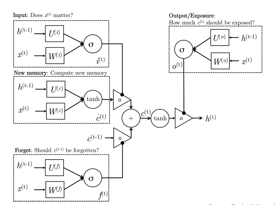
Figure 5: Schematic representation of the LSTM architecture. The diagram depicts the flow of data through the input, forget, output gates, and the cell state, emphasizing the modular nature of LSTM units.

Each block of the LSTM diagram corresponds to a specific function within the unit:

The input gate determines the extent to which new data ( $xt$ ) affects the state of the memory cell.
The forget gate decides what portions of the existing memory ( $ct−1$ ) should be retained or discarded.
The output gate controls how the memory cell’s state ( $ct$ ) influences the output ( $ht$ ).
The cell state ( $ct$ ) is updated based on the inputs from these gates, ensuring the retention of long-term dependencies.

This visual representation serves as an intuitive guide for understanding the internal workings of LSTM networks, particularly how they selectively remember and forget information to maintain robustness in processing sequential data.

4.7.7 Training Long Short-Term Memory Networks

Training Long Short-Term Memory (LSTM) networks is a nuanced process that is essential for these models to effectively learn from sequence data. The cornerstone of LSTM training is the method known as Backpropagation Through Time (BPTT). This technique involves unrolling the LSTM network through time and applying the traditional backpropagation algorithm. It meticulously computes the gradients of the loss function with respect to the weights of the network, which are based on the output sequence. These gradients are then used to update the weights, thereby incrementally improving the LSTM’s performance on the task.

However, training LSTMs is not without its challenges. One major issue is the vanishing gradients problem, where gradients become infinitesimally small as they are propagated back through the timesteps, leading to negligible changes in the weights and consequently, stagnant learning. The opposite scenario can occur with exploding gradients, where the gradients become excessively large, causing the model parameters to oscillate or diverge wildly with each update.

To combat these issues, several techniques have been developed. Gradient clipping is a straightforward yet effective strategy that prevents the gradients from becoming too large, simply by capping them to a maximum value. Weight initialization also plays a pivotal role; starting the training process with appropriately scaled weights can significantly mitigate the vanishing gradient problem. Additionally, the adoption of advanced optimizers such as Adam or RMSprop, which adjust the learning rates based on the evolution of gradients, can lead to more stable and efficient training. Lastly, regularization techniques like dropout, when applied to the inputs and outputs of the LSTM cells, can help in preventing overfitting to the training data.

Each of these methods contributes to the robustness of LSTM training, allowing these networks to learn effectively from complex, lengthy sequences and perform exceptionally well on a wide range of sequence modeling tasks.

4.7.8 LSTM in Economics and Finance

Long Short-Term Memory (LSTM) networks have revolutionized the field of economic and financial analysis. With their exceptional ability to model and predict complex sequential data, LSTM has become a cornerstone in forecasting and decision-making processes within these sectors.

Forecasting Economic Indicators: Economists utilize LSTM networks to predict critical economic indicators such as GDP growth rates, inflation, and unemployment rates. By analyzing historical data, LSTM helps in decoding economic cycles, which is invaluable for developing future economic policies and preparing for cyclical downturns or upturns.

Financial Market Analysis: In the realm of finance, LSTM offers significant advantages in predicting stock prices, market trends, and volatility. Their proficiency in analyzing sequential market data allows for the modeling of complex market behaviors, which is instrumental in risk management and investment strategy development.

Credit Risk Modeling: Credit risk assessment is another area where LSTM demonstrates its prowess. By analyzing the sequential financial activities of borrowers, these networks can predict future credit behaviors with a high degree of accuracy, which is crucial for identifying potential default risks and making informed lending decisions.

Algorithmic Trading: The use of LSTM in algorithmic trading is transforming the industry. These networks can decipher patterns in high-frequency trading data, enabling traders to develop automated strategies that can adapt to market changes, providing a substantial competitive advantage.

Time Series Forecasting in Various Financial Domains: LSTM is versatile and can be applied to a broad spectrum of financial domains. Whether it’s predicting interest rates or forecasting commodity prices, LSTM is adept at capturing the underlying patterns in time series data. Its ability to remember and utilize long-term dependencies equips it to handle the seasonality and trends typical of financial time series data effectively.

In summary, the robustness of LSTM in sequence modeling and its capacity to remember information over long periods make it an indispensable tool for economic and financial forecasting. These capabilities allow for a deeper understanding of economic and financial phenomena, leading to more accurate predictions and better strategic decisions.

4.8 Natural Language Processing (NLP) Models Google Colab

4.8.1 Introduction

In the realm of financial forecasting, the integration of Artificial Intelligence (AI) technologies, particularly Long Short-Term Memory (LSTM) networks and sentiment analysis, has marked a significant evolutionary step. This subsection delves into the profound impact of news sentiment on stock returns, exploring how AI-driven Natural Language Processing (NLP) techniques assess and interpret the mood and opinions embedded within financial news. The predictive power of sentiment analysis, when harnessed effectively, can lead to notable stock price fluctuations in response to the collective market sentiment.

Furthermore, the application of advanced AI techniques, including LSTM networks, underscores the potential to process and analyze time-series data of sentiment scores, offering a nuanced approach to predictive analytics in finance. These methodologies not only navigate the challenges posed by the inherent sarcasm, ambiguity, and context variability in news content but also seamlessly integrate with financial algorithms to enhance forecasting accuracy.

The transition from news sentiment to actionable market predictions involves a systematic approach to data collection, sentiment scoring, and the utilization of sentiment data within LSTM networks to forecast stock returns. This process highlights the crucial role of sentiment analysis in bridging the gap between raw news content and actionable financial insights.

Illustrative case studies and practical applications of these AI-driven approaches offer concrete evidence of their effectiveness in predicting market movements. Such examples not only demonstrate the practical utility of sentiment analysis in shaping investment strategies but also pave the way for discussions on future trends and the exploration of next-generation technologies in market analysis.

This introduction sets the stage for a comprehensive exploration of AI-driven financial forecasting, emphasizing the transformative potential of LSTM networks and sentiment analysis in revolutionizing the financial industry.

4.8.2 Extracting Sentiment from Financial News

The integration of Natural Language Processing (NLP) into the analysis of financial markets signifies a paradigm shift in how data is interpreted at scale. NLP facilitates the automated understanding of human language, a feature that proves invaluable when sifting through the extensive volumes of financial news for sentiment analysis. This analysis process begins with tokenization, the segmentation of text into manageable units or tokens, which forms the foundation for subsequent analytical techniques aimed at deriving sentiment from textual data.

The toolbox for NLP encompasses a range of technologies, from the foundational libraries like NLTK and spaCy, which provide the means for basic text manipulation (e.g., tokenization, stemming), to more sophisticated frameworks such as TensorFlow and PyTorch. These advanced platforms enable the development and training of deep learning models, including those based on LSTM networks, designed to interpret complex patterns in sentiment data.

A pivotal component of sentiment analysis is the quantification of sentiment, transforming qualitative textual cues into quantifiable scores. This quantification is facilitated by sentiment lexicons like VADER and AFINN, which attribute sentiment scores to specific lexical items. Beyond lexicons, machine learning models trained on labeled datasets offer a dynamic approach to sentiment classification, categorizing sentiments as positive, negative, or neutral based on the analysis of text. These models, nurtured by the preparatory work of tokenization and leveraging the computational power of the aforementioned technologies, stand at the forefront of market sentiment analysis, offering nuanced insights into the fluctuating moods of financial markets.

This overview underscores the essential role of NLP in distilling sentiment from financial news, highlighting the foundational techniques, critical tools, and methods employed in the quantification of sentiment. As financial markets evolve, the application of NLP in sentiment analysis remains a cornerstone of financial forecasting, enabling analysts to leverage textual data for predictive insights with unprecedented precision and scale.

4.8.3 Building LSTM Models for Financial Forecasting

The advent of Long Short-Term Memory (LSTM) networks represents a significant leap forward in financial forecasting, offering a robust methodology for capturing the intricate patterns within time-series data. The development of these models entails a comprehensive approach, starting with the meticulous collection and preprocessing of data, through to the nuanced design of the LSTM architecture itself.

Data Collection and Preprocessing
The foundation of any predictive model lies in the quality and relevance of the data it analyzes. In the context of financial forecasting, this data encompasses a broad spectrum, from financial news articles and reports to the dynamic landscape of social media. The challenges inherent in this process—namely the volume, velocity, variety, and veracity of data—necessitate a rigorous preprocessing regimen. Techniques such as tokenization, noise removal, and normalization are employed to refine this data, ensuring it is in a form conducive to analysis.

Structuring Time-Series Data
A critical step in preparing data for LSTM models involves the alignment of sentiment scores derived from news content with historical stock price movements. This process creates a chronological sequence of data points, facilitating a temporal analysis that is sensitive to the unfolding of market events over time.

Feature Engineering for LSTM Inputs
The predictive capability of LSTM models is significantly enhanced through the careful selection and incorporation of features. Sentiment scores, market indicators, and other pertinent financial metrics are integrated, offering a multifaceted view of the factors influencing stock prices. This stage is crucial for tailoring the model to recognize and respond to the specific dynamics of the financial market.

Designing LSTM Models
The architecture of LSTM models is specifically tailored to address the challenges of financial forecasting. By capturing long-term dependencies within the data, these models can anticipate future stock returns with a remarkable degree of accuracy. Optimizing the model parameters further refines this process, enhancing the model’s ability to make precise predictions.

This overview encapsulates the intricate process of building LSTM models for financial forecasting. From the initial stages of data collection and preprocessing to the sophisticated engineering of features and model architecture, each step is instrumental in shaping the predictive prowess of LSTM networks. As we venture into the future, the continued refinement and application of these models hold the promise of revolutionizing financial analytics, offering insights of unprecedented depth and accuracy.

4.8.4 Optimizing LSTM for Financial Insights

Long Short-Term Memory (LSTM) networks represent a cornerstone in the advancement of financial forecasting, offering sophisticated mechanisms to interpret and predict market movements. The architecture of LSTM models is meticulously designed to handle the complexities of financial time-series data, ensuring a nuanced analysis that accounts for both short-term fluctuations and long-term trends.

LSTM Model Architecture:
At the foundation of an LSTM model lies its distinctive architecture, composed of various layers each tailored to perform specific functions:
- Input Layers process raw numerical data, transforming sentiment scores and market indicators into a format suitable for analysis.
- LSTM Layers serve as the model’s core, where time-series data is scrutinized to identify and learn from patterns of market behavior.
- Dropout Layers are strategically implemented to mitigate the risk of overfitting, ensuring the model’s robustness by randomly omitting subsets of features.
- Output Layers culminate the analytical process, delivering predictions on future stock prices or market movements based on the insights garnered through the LSTM network.

Integrating News Sentiment:
Incorporating sentiment analysis into the forecasting model amplifies its accuracy. By analyzing sentiment scores derived from financial news alongside historical stock data, the model gains an enhanced perspective, allowing for more accurate predictions that reflect both quantitative trends and qualitative insights from the market.

Training the LSTM Model:
The training process is critical to the model’s success. It involves:
- Data Splitting to segregate the dataset into distinct sets for training, validation, and testing.
- Normalization of input data to standardize the scale across different metrics, improving the model’s learning efficiency.
- Selecting Loss Functions and Optimizers to fine-tune the model, minimizing prediction errors while enhancing the rate and quality of learning.

Evaluating Model Performance:
Performance evaluation employs various metrics to assess the model’s predictive power and reliability. Accuracy, precision, recall, and F1-score are among the metrics used to quantify how well the model predicts stock returns, offering insights into its effectiveness and areas for improvement.

This section explores the nuanced process of optimizing LSTM models for financial forecasting, emphasizing the architectural design, integration of news sentiment, training methodologies, and evaluation criteria. As financial markets continue to evolve, the refinement and application of LSTM models are poised to play a pivotal role in shaping the future of financial analysis.

4.8.5 Advancing Financial Predictions with LSTM

Long Short-Term Memory (LSTM) networks have significantly impacted financial forecasting, offering deep insights into future market movements through the sophisticated analysis of time-series data. This section delves into the construction and operation of LSTM models, particularly focusing on their architecture, integration with sentiment analysis, and the critical process of model training.

The architecture of an LSTM model is meticulously designed to process complex financial data efficiently. At the initial stage, input layers handle raw numerical data, including sentiment scores derived from financial news and various market indicators. This is followed by the LSTM layers, which are pivotal in analyzing time-series data, capturing both short-term fluctuations and long-term trends. To enhance model reliability and prevent overfitting, dropout layers are employed, randomly excluding features during the training phase to ensure the model’s generalizability. The architecture culminates in the output layers, which generate predictions about future stock prices or market movements. Integral to enhancing the model’s predictive accuracy is the integration of news sentiment, where sentiment scores from financial news are merged with traditional stock data, providing a comprehensive view of potential market drivers.

Training the LSTM model is a critical phase where the constructed model is refined to accurately predict market trends. This involves data preparation, where collected data is divided into training, validation, and test sets, and normalized to facilitate efficient model training. The optimization process then selects appropriate loss functions and optimizers, fine-tuning the model to minimize prediction errors and enhance its forecasting capabilities.

Through the integration of LSTM networks and sentiment analysis, financial forecasting is poised for a significant transformation. These technologies offer the potential to decode complex market signals and predict future trends with unprecedented accuracy, marking a new era in financial analysis.

4.8.6 Evaluating LSTM Models for Stock Prediction

The evaluation of Long Short-Term Memory (LSTM) models in the domain of stock prediction is a meticulous process that necessitates the use of specific metrics and considerations to ensure model reliability and effectiveness. This subsection explores the fundamental metrics for accuracy assessment, the critical balance between overfitting and underfitting, and a comparative analysis with traditional forecasting models.

Metrics for Accuracy Assessment: Accuracy assessment in financial forecasting models, particularly those predicting stock prices, relies on several key metrics:
- Mean Squared Error (MSE) quantifies the average of the squares of the errors, essentially measuring the average squared difference between the estimated values and what is estimated.
- Mean Absolute Error (MAE) computes the average of the absolute differences between predictions and actual outcomes, offering a measure less sensitive to outliers than MSE.
- R-squared (R²) indicates the proportion of the variance for a dependent variable that’s predicted from the independent variables, providing insight into the goodness of fit.

Overfitting vs. Underfitting: Model reliability hinges on striking a perfect balance between overfitting and underfitting:
- Overfitting occurs when a model learns the detail and noise in the training data to the extent that it negatively impacts the performance of the model on new data. Techniques like introducing dropout layers or increasing the dataset size are common mitigation strategies.
- Underfitting is observed when a model cannot capture the underlying trend of the data. Enhancing model complexity or improving feature engineering practices are typical responses to underfitting.

Comparative Analysis: A comprehensive evaluation of LSTM models also involves comparing their performance against traditional time-series forecasting models, such as ARIMA (Autoregressive Integrated Moving Average) and VAR (Vector Autoregression). Criteria for this comparison often include predictive accuracy, computational efficiency, and the model’s aptitude for handling non-linear data.

This thorough approach to evaluating LSTM models for stock prediction not only underscores the precision and reliability of these models but also highlights their comparative advantages over traditional forecasting methods, marking a significant advancement in the field of financial analytics.

4.8.7 Challenges and Future of AI in Financial Forecasting

As the financial industry increasingly leans on Artificial Intelligence (AI) for market forecasting, several challenges and ethical considerations emerge, alongside promising future directions for this technology.

Limitations of LSTM Models

While Long Short-Term Memory (LSTM) networks have proven to be powerful tools for analyzing financial time-series data, they are not without their limitations. The quality and relevance of historical data are paramount; LSTM models heavily rely on this data to make predictions, making them susceptible to the garbage-in-garbage-out principle. Market efficiency presents another challenge, as LSTM models, like all predictive models, struggle to forecast markets that efficiently incorporate all available information into asset prices. External factors, such as geopolitical events or sudden market shocks, which are not captured in past data trends, further complicate prediction accuracy.

Ethical Considerations in Automated Trading

The rise of automated trading systems powered by AI algorithms brings to the forefront significant ethical considerations. Transparency in how these algorithms make decisions is crucial for trust and accountability. Determining who is responsible for the consequences of algorithmic decisions is another critical issue. As these technologies advance, ensuring regulatory compliance becomes increasingly complex, necessitating continuous adaptation to evolving legal standards.

Future Directions in AI-Driven Forecasting

Despite these challenges, the future of AI in financial forecasting is bright, with innovative technologies continually being explored to address current limitations and introduce new capabilities. The development of models that can incorporate real-time data and understand complex market dynamics promises potential disruptions in the field. Furthermore, the financial industry anticipates the evolution of regulatory and ethical frameworks in response to advancements in AI and machine learning, ensuring that these technologies are used responsibly and effectively.

This subsection delves into the nuanced challenges and considerations facing AI in financial forecasting, underscoring the importance of addressing these issues while also highlighting the optimistic outlook for future advancements in the field.

4.8.8 Wrapping Up: The Future of AI in Financial Forecasting

As we conclude our exploration of AI in financial forecasting, we reflect on the journey through the sophisticated realms of Long Short-Term Memory (LSTM) networks and sentiment analysis. This section recaps the foundational concepts, evaluates the transformative impact of these technologies on financial forecasting, and opens a dialogue on the broader applications and future directions.

Recap of Key Concepts:
The discourse has spanned the intricate architecture and applications of LSTM networks, adept at unraveling complex time-series data patterns for stock return prediction. Sentiment analysis has been spotlighted for its capacity to enrich financial models with nuanced insights derived from news and social media. Critical challenges such as ensuring data quality, navigating market efficiency, addressing ethical considerations, and maintaining the delicate equilibrium between overfitting and underfitting have been thoroughly reviewed.

Revolutionizing Financial Forecasting:
The synergy between LSTM networks and sentiment analysis has been emphasized as a robust framework capable of anticipating market movements with unprecedented precision. The amalgamation of these AI technologies promises to usher in a new era of financial forecasting, characterized by models that are not only more accurate but also dynamic and insightful.

Open Discussion:
In the spirit of continuous exploration and learning, we invite inquiries, comments, and feedback to further our collective understanding. The discussion extends beyond the confines of stock prediction, contemplating the vast potential of AI in finance. Areas ripe for exploration include risk management, fraud detection, and personalized financial advice, each offering new horizons for the application of AI technologies.

As we stand on the cusp of innovation, the future of AI in financial forecasting shines brightly, heralding a paradigm shift in how financial markets are analyzed and understood. The path forward is marked by the potential for groundbreaking developments that promise to redefine the landscape of financial analysis.

Chapter 4: Predictive Models in Economic and Social Issues

4.1 Introduction

4.2 Linear Regression Models Google Colab CheckMe!

4.2.1 Simple Linear Regression

4.2.1.1 Example

4.2.2 Multiple Linear Regression

4.2.2.1 Example

4.2.3 Model Evaluation

4.2.3.1 Mean Squared Error (MSE)

4.2.3.2 Root Mean Squared Error (RMSE)

4.2.3.3 (Coefficient of Determination)

4.2.3.4 Example of Model Evaluation

4.2.4 Conclusion

4.3 Time Series Forecasting Models Google Colab CheckMe!

4.3.1 Recursive Forecasting

4.3.2 Rolling Window Forecasting

4.3.3 Stationarity

4.3.4 Tests for Stationarity

4.3.5 Differencing

4.3.6 Types of Time Series Forecasting Models

4.3.6.1 Autoregression (AR)

4.3.6.2 Moving Average (MA)

4.3.6.3 Autoregressive Moving Average (ARMA)

4.3.6.4 Autoregressive Integrated Moving Average (ARIMA)

4.3.6.5 Autoregressive Distributed Lag (ARDL)

4.3.6.6 Seasonal Decomposition of Time Series (STL)

4.3.6.7 Exponential Smoothing (ETS) Model

4.3.6.8 Vector Autoregression (VAR)

4.3.7 Conclusion for Time Series Forecasting

4.4 Prophet Forecasting Google Colab CheckMe!

4.4.1 Model Components

4.4.2 Trend Component

4.4.2.1 Piecewise Linear Trend

4.4.2.2 Logistic Growth Trend

4.4.3 Seasonality Component

4.4.4 Holiday Component

4.4.5 Error Term

4.4.6 Model Fitting

4.4.7 Forecasting with Prophet

4.4.8 Example: Forecasting Retail Sales

4.4.9 Step 1: Prepare the Data

4.4.10 Step 2: Fit the Model

4.4.11 Step 3: Make Predictions

4.4.12 Conclusion

4.5 Neural Networks and Deep Learning CheckMe!

4.5.1 Introduction to Neural Networks and Deep Learning

4.5.2 What are Neural Networks?

4.5.3 Structure of a Neural Network

4.5.4 Mathematical Formulation of a Neural Network

4.5.5 Activation Functions in Neural Networks

4.5.6 Understanding Parameter Estimation in Neural Networks

4.5.7 Fitting Neural Networks

4.5.8 Empowering Economics and Finance with Neural Networks

4.6 Recurrent Neural Networks Google Colab CheckMe!

4.6.1 Recurrent Neural Networks: Overview and Applications

4.6.2 The Structure of Simple Recurrent Neural Networks

4.6.3 RNN Mathematical Framework

4.6.4 Loss Function in RNNs for Regression Problems

4.6.5 Application of RNNs in Financial Time Series Forecasting

4.7 Long Short-Term Memory (LSTM) Networks Google Colab CheckMe!

4.7.1 Overview of LSTM

4.7.2 LSTM Architecture

4.7.3 Gate Operations in LSTM

4.7.4 Output Gate, Cell State Update, and Activation Functions

4.7.5 LSTM Components and Activation Functions

4.7.6 Visualizing the LSTM Architecture

4.7.7 Training Long Short-Term Memory Networks

4.7.8 LSTM in Economics and Finance

4.8 Natural Language Processing (NLP) Models Google Colab CheckMe!

4.8.1 Introduction

4.8.2 Extracting Sentiment from Financial News

4.8.3 Building LSTM Models for Financial Forecasting

4.8.4 Optimizing LSTM for Financial Insights

4.8.5 Advancing Financial Predictions with LSTM

4.8.6 Evaluating LSTM Models for Stock Prediction

4.8.7 Challenges and Future of AI in Financial Forecasting

4.8.8 Wrapping Up: The Future of AI in Financial Forecasting

Ask ChatGPT

4.2 Linear Regression Models Google Colab

4.2.3.3 $R2$ (Coefficient of Determination)

4.3 Time Series Forecasting Models Google Colab

4.4 Prophet Forecasting Google Colab

4.5 Neural Networks and Deep Learning

4.6 Recurrent Neural Networks Google Colab

4.7 Long Short-Term Memory (LSTM) Networks Google Colab

4.8 Natural Language Processing (NLP) Models Google Colab