Chapter 2: Causal Estimation Techniques

2.1 Instrumental
Variables (IV)
Google Colab
2.1.1
Introduction to Instrumental Variables
Instrumental Variables (IV) stand as a pivotal econometric tool aimed at estimating causal relationships in scenarios where conducting controlled experiments is either not feasible or ethical considerations preclude their use. This comprehensive approach not only introduces the concept of IV but also elaborates on its purpose, delineates the sources of endogeneity that IV methods are designed to address, and elucidates how IV methods furnish solutions to these intricate problems.
Instrumental Variables (IV) are employed in statistical analyses to deduce causal relationships under circumstances where controlled experiments are untenable. The quintessential goal behind the utilization of IV methods is to confront and resolve endogeneity issues within econometric models, thereby facilitating a more precise and accurate inference of causality. The challenge of endogeneity emerges from various quarters, each complicating the accurate estimation of causal effects. Primarily, these sources include:
- Omitted Variable Bias: This occurs when a model does not include one or more relevant variables, leading to biased and inconsistent estimates.
- Measurement Error: Errors in measuring explanatory variables can introduce biases and inconsistencies in the estimations, distorting the true relationship between variables.
- Simultaneity: This arises when the causality between variables is bidirectional, complicating the determination of the direction of the causal relationship.
Instrumental Variables methods leverage an external source of variation that influences the endogenous explanatory variable yet remains uncorrelated with the error term within the model. By capitalizing on this external variation, IV methods adeptly navigate through the aforementioned issues of endogeneity, offering a more dependable estimation of causal effects. A notable example illustrating the application of IV is in estimating the impact of education on earnings. The selection of an instrument, such as proximity to colleges, introduces a variation in educational attainment that is exogenous to an individual’s potential earnings, thus permitting an unbiased estimation of the causal effect of education on earnings.
2.1.2 Comparing
Instrumental Variables to Randomized Controlled Trials
Randomized Controlled Trials (RCTs) are deemed the gold standard for causal inference due to their method of randomly assigning treatments to subjects, allowing for the direct observation of causal effects. This random assignment ensures that both the treatment and control groups are statistically equivalent across all characteristics, both observable and unobservable, thus providing clear and unbiased estimates of causal effects.
However, there are scenarios where RCTs are not feasible due to practical limitations, ethical concerns, or the inherent nature of the treatment variable. In such cases, Instrumental Variables (IVs) offer an alternative method for causal inference. IVs are employed when conducting controlled experiments is impractical or unethical. They rely on natural or quasi-experiments and require strong assumptions regarding the instrument’s relevance to the endogenous explanatory variable and its exogeneity to the error term.
The primary distinctions between IVs and RCTs lie in the approach to controlling for confounders. While RCTs achieve this through randomization, IV methods exploit external instruments that mimic random assignment, albeit without direct control by the researcher. This makes IVs particularly useful in situations where:
- Conducting RCTs is impractical, unethical, or excessively costly.
- The effects of variables that cannot be manipulated or randomly assigned are being studied, such as age or geographical location.
- Addressing specific endogeneity issues in observational data that RCTs cannot resolve.
Both RCTs and IVs are instrumental in the causal inference toolbox, each with its unique set of strengths and applicable scenarios. The choice between using an IV approach over RCTs hinges on the research context, the feasibility of experiments, and the nature of the variables involved.
2.1.3 The IV
Estimation Idea
The Instrumental Variables (IV) approach serves as a pivotal solution to the endogeneity problem within econometric analysis. Endogeneity often complicates causal inference, rendering conventional estimation techniques ineffective. IV estimation intervenes by utilizing an instrument—a variable that is correlated with the endogenous explanatory variables yet uncorrelated with the error term in the regression model. This unique characteristic of the instrument allows for the isolation and measurement of the causal impact of the explanatory variable on the outcome.
Conceptual Framework: At its core, IV estimation facilitates causal inference through the exploitation of variation in the explanatory variable that is directly associated with the instrument but remains independent of the confounding factors encapsulated in the error term. This methodological framework ensures that the estimated effects are devoid of bias arising from omitted variables or measurement errors, common sources of endogeneity.
Graphical Illustration: Consider a simplified representation where:
-
 denotes the
instrument whose primary role is to affect the endogenous variable
(
denotes the
instrument whose primary role is to affect the endogenous variable
( ) without
directly influencing the outcome variable (
) without
directly influencing the outcome variable ( ).
).
-
 represents the
endogenous explanatory variable that is presumed to causally
impact
represents the
endogenous explanatory variable that is presumed to causally
impact  , the
outcome of interest.
, the
outcome of interest.
-
The causal pathway from
 to
to
 is mediated
entirely through
is mediated
entirely through
 , underscoring
the instrument’s indirect influence on the outcome.
, underscoring
the instrument’s indirect influence on the outcome.
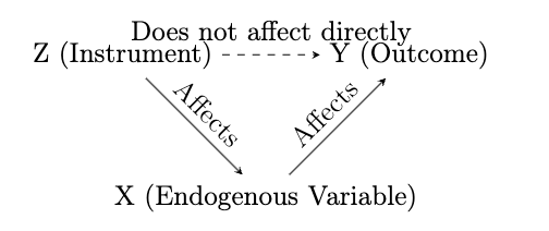
The accompanying diagram visualizes these relationships,
highlighting the instrument’s (Z) effect on the endogenous variable
(X) and, subsequently, on the outcome variable (Y), while
emphasizing the absence of a direct link from
 to
to
 . This graphical
representation aids in conceptualizing the instrumental variable as
a lever to uncover the causal effect of
. This graphical
representation aids in conceptualizing the instrumental variable as
a lever to uncover the causal effect of
 on
on
 , circumventing
the pitfalls of endogeneity.
, circumventing
the pitfalls of endogeneity.
This section underscores the theoretical underpinnings and practical implications of IV estimation, illustrating its utility in empirical research where experimental designs are infeasible. Through this method, researchers are equipped to forge a path towards robust causal inference, navigating the challenges posed by endogenous relationships within their analytical frameworks.
2.1.4 Key
Assumptions and Conditions for Valid Instrumental Variables
Instrumental Variables (IV) estimation stands as a cornerstone econometric method for addressing endogeneity, enabling researchers to uncover causal relationships where direct experimentation is impractical. The efficacy of this approach, however, hinges on the satisfaction of several critical assumptions. These assumptions ensure that the instruments employed can legitimately serve as proxies for the endogenous explanatory variables, thereby providing unbiased and consistent estimators of causal effects.
First Assumption: Relevance The relevance condition necessitates a strong correlation between the instrument and the endogenous explanatory variable. This relationship is crucial as it underpins the instrument’s ability to meaningfully influence the endogenous variable, thereby offering a pathway to identify the causal effect of interest. Mathematically, this assumption is expressed as:

where the covariance between the instrument and the endogenous variable must be non-zero. This statistical relationship validates the instrument’s capacity to induce variations in the endogenous explanatory variable that are essential for IV estimation.
Second Assumption: Exogeneity The assumption of exogeneity asserts that the selected instrument must be uncorrelated with the error term in the regression equation. This condition is vital to ensure that the instrument does not capture any of the omitted variable biases that might otherwise contaminate the estimations. The mathematical representation of this assumption is:

where  denotes
the error term. Fulfillment of this criterion guarantees that the
instrument’s variation is purely exogenous, thereby facilitating a
clear isolation of the causal impact of the endogenous variable on
the outcome.
denotes
the error term. Fulfillment of this criterion guarantees that the
instrument’s variation is purely exogenous, thereby facilitating a
clear isolation of the causal impact of the endogenous variable on
the outcome.
Overidentification and Multiple Instruments In scenarios where researchers deploy multiple instruments, each instrument must independently satisfy both the relevance and exogeneity conditions. Additionally, the instruments should not be perfectly correlated with each other, ensuring that each offers distinct information about the endogenous variable. The Sargan-Hansen test provides a mechanism to test for overidentification, verifying that the instruments as a collective are valid and do not overfit the model.
Note: Adherence to these key assumptions is imperative for the integrity of IV estimation. Violations may lead to biased and inconsistent results, emphasizing the necessity for meticulous instrument selection and rigorous validation processes. The careful application of these principles ensures that IV methods yield reliable insights into causal relationships, thereby enhancing the robustness of econometric analysis.
2.1.5
Identification with Instrumental Variables
Identification plays a pivotal role in the utilization of Instrumental Variables (IV) within econometric analysis. Specifically, identification refers to the capacity to accurately estimate the causal impact of an independent variable on a dependent variable by harnessing the exogenous variation induced by the IV. This concept is foundational in ensuring that the causal inferences drawn from IV estimations are valid and reliable.
Conditions for Robust Identification: Achieving proper identification with IVs necessitates adherence to several critical conditions, each designed to validate the instrument’s effectiveness in isolating the true causal relationship:
- Instrument Exogeneity: The cornerstone of IV identification is the requirement that the instrument must not share any correlation with the error term in the regression model. This ensures that the instrument’s influence on the dependent variable is channeled exclusively through its correlation with the endogenous independent variable, thereby eliminating concerns of omitted variable bias influencing the estimates.
- Instrument Relevance: Moreover, for an IV to be considered valid, it must exhibit a strong correlation with the endogenous independent variable. This condition, known as instrument relevance, guarantees that the IV introduces sufficient exogenous variation to effectively identify the causal effect in question.
- Single Instrument Single Endogenous Variable: In scenarios involving a single instrument and a single endogenous variable, the IV methodology primarily identifies the Local Average Treatment Effect (LATE). This specific effect pertains to the subset of the population whose treatment status (i.e., the endogenous variable) is influenced by the instrument.
- Multiple Instruments: The introduction of multiple instruments potentially broadens the scope of identification beyond LATE, facilitating a more comprehensive understanding of the causal effect across different segments of the population. However, this extension is contingent upon the validity of the instruments and adherence to the above conditions.
Importance of Proper Identification: The essence of leveraging IVs in econometric analysis rests on the premise of proper identification. It is this principle that distinguishes genuine causal relationships from mere correlations or associations marred by endogeneity. Ensuring that the conditions for identification are met is not merely a technical exercise but a fundamental prerequisite for the empirical credibility of IV estimation, underscoring the nuanced complexities inherent in causal inference.
2.1.6
Two-Stage Least Squares (2SLS) Methodology
The Two-Stage Least Squares (2SLS) methodology emerges as a cornerstone technique in the realm of econometrics, specifically tailored for instrumental variables estimation to tackle the pervasive issue of endogeneity. This method delineates a systematic approach to estimating the causal impact of an independent variable on a dependent variable by leveraging an instrument that remains uncorrelated with the error term, thereby circumventing the biases associated with endogeneity.
Operational Stages of 2SLS: The implementation of 2SLS is methodically divided into two distinct stages, each serving a unique purpose in the estimation process:
- First Stage: Initially, the focus is on regressing the endogenous independent variable against the instrumental variable(s) alongside any exogenous variables present within the model. This stage is instrumental in deriving the predicted values for the endogenous variable, which are ostensibly purged of the endogeneity bias. The primary objective here is to substitute the original endogenous variable with its predictions based on the instrumental variables, ensuring these estimates are devoid of the original endogeneity concerns.
- Second Stage: Subsequently, the analysis proceeds to regress the dependent variable on the predicted values obtained from the first stage, in addition to incorporating any other exogenous variables. This crucial stage aims to quantify the causal effect of the endogenous variable on the dependent variable, now equipped with a predictor that is cleansed of endogeneity. The essence of this stage lies in its capacity to furnish an estimation of the causal relationship, effectively addressing the initial endogeneity issue.
Significance of 2SLS in Empirical Research: The advent of the 2SLS method marks a significant milestone for empirical investigations, particularly in scenarios where deploying natural experiments or conducting randomized control trials pose substantial challenges. By offering a viable and robust alternative to ordinary least squares (OLS) regression in the face of endogeneity, 2SLS enhances the reliability and validity of causal inferences drawn from econometric analyses.
Example 1: IV in Regression Analysis
This section provides a comprehensive look at employing Instrumental Variables (IV) in regression analysis to assess the causal influence of education on earnings.
Problem Definition:
-
Aim: Accurately estimate the causal effect of education (
 ) on earnings (
 ), mitigating endogeneity issues.
Regression Model:
| (1) |

Endogeneity Challenge:
-
 could be endogenously correlated with
 ,
potentially due to omitted variables, measurement error, or
reverse causality, risking bias in OLS estimates.
,
potentially due to omitted variables, measurement error, or
reverse causality, risking bias in OLS estimates.
Instrumental Variable Strategy:
-
Chosen Instrument: Proximity to the nearest college (Distance to College), presumed to affect
 without directly influencing
 ,
except via
,
except via
 .
.
Two-Stage Least Squares (2SLS) Method:
-
First Stage: Estimate
 as a function of
 and other exogenous variables:
(2) -
Second Stage: Regress
 on
the predicted values of
on
the predicted values of
 from Equation (2), isolating the causal effect:
(3)


Equations (2) and (3) elaborate on the 2SLS process, elucidating the mechanism to
address the endogeneity of
 in
estimating its impact on
in
estimating its impact on
 .
.
Conclusion: Implementing the 2SLS technique, with Distance to College as an instrumental variable, enables a more accurate estimation of the causal effect of education on earnings, effectively handling the endogeneity bias and enhancing result interpretability.
Example 2: IV in Regression Analysis
This example illustrates the use of Instrumental Variables (IV) in regression analysis to estimate the causal effect of police presence on crime rates, particularly addressing endogeneity concerns.
Problem Statement:
-
Objective: Estimate the causal impact of police presence (
 ) on crime rates (
 ).
).
-
Regression Model:
(4) -
Concern:
 may be endogenously correlated with
 ,
complicating causal interpretation.
,
complicating causal interpretation.

Instrumental Variable Solution:
-
Proposed Instrument: Political changes, assumed to influence
police allocation and thereby
 , independent of the crime rate.
Two-Stage Least Squares (2SLS) Approach:
-
First Stage: Predict
 as a function of the instrumental variable and possibly other
exogenous covariates.
as a function of the instrumental variable and possibly other
exogenous covariates.
(5) -
Second Stage: Use the predicted values of
 (
( ) from the first stage to estimate its effect on
 .
.
(6)


Equations (5) and (6) form the core of the 2SLS methodology, providing a framework to
estimate the causal effect of
 on
on
 while
mitigating endogeneity bias.
while
mitigating endogeneity bias.
Conclusion: The application of the 2SLS method with an appropriate instrumental variable allows for a more accurate and causally interpretable estimate of the impact of police presence on crime rates, highlighting the importance of addressing endogeneity in econometric analysis.
2.1.7 Testing
IV Assumptions, Validity, and Challenges
Instrumental variables (IV) analysis is a critical method in econometrics for addressing endogeneity issues. Testing the assumptions and validity of IVs, along with acknowledging their challenges and limitations, is essential for credible causal inference.
Testing IV Assumptions and Validity. The relevance of IVs is initially assessed through F-statistics, which help to check the strength of the instrument. A low F-statistic suggests that the instrument may be weak, potentially leading to unreliable estimates. For a more direct assessment of instrument strength, specific weak instrument tests are applied to evaluate the significant correlation between the instrument and the endogenous variable.
In addition to relevance, the exogeneity of IVs is crucial. Overidentification tests are utilized when multiple instruments are available, allowing researchers to check if the instruments are uncorrelated with the error term, thus satisfying the exogeneity condition. Moreover, Hansen’s J statistic offers a formal approach to test the overall validity of the instruments by assessing both relevance and exogeneity assumptions together.
Challenges and Limitations of Using IV. Identifying valid instruments that meet both relevance and exogeneity conditions is a practical challenge in applied research. Weak instruments, if not adequately tested, can lead to biased and inconsistent estimates, undermining the reliability of the causal inference. Even with strong instruments, incorrect model specifications or violations of the IV assumptions can result in biased estimates, highlighting the importance of rigorous testing and validation in IV analysis.
This comprehensive approach to testing IV assumptions, along with a critical understanding of the potential challenges and pitfalls, ensures the robustness and credibility of the causal inferences drawn from econometric analyses.
IV Applications in Various Fields
Economic History and Development Economics: The Long-Term Effects of Africa’s Slave Trades, Nathan Nunn, The Quarterly Journal of Economics, 2008
- Objective: Examine the impact of Africa’s slave trades on its current economic underdevelopment.
- Methodology Instrument: Use of shipping records and historical documents to estimate the number of slaves exported from each African country as an instrumental variable.
- Reason: The historical intensity of slave trades is employed to identify the causal effect on present-day economic performance, isolating the impact from other confounding factors.
- Data: Compilation of slave export estimates from various sources, including the Trans-Atlantic Slave Trade Database, and data on slave ethnicities to trace the origins of slaves.
- Results: Finds a robust negative relationship between the number of slaves exported and current economic performance, suggesting a significant adverse effect of the slave trades on economic development.
Labor Economics: Does Compulsory School Attendance Affect Schooling and Earnings?, Joshua D. Angrist and Alan B. Krueger, The Quarterly Journal of Economics, 1991
- Objective: Investigate the effect of compulsory school attendance laws on educational attainment and earnings.
- Methodology & Instrument: Utilization of quarter of birth as an instrumental variable for education, exploiting the variation in educational attainment induced by compulsory schooling laws.
- Reason: Season of birth affects educational attainment due to school entry age policies and compulsory attendance laws, providing a natural experiment for estimating the impact of education on earnings.
- Data: Analysis of U.S. Census data to examine the relationship between education, earnings, and season of birth.
- Results: The study finds that compulsory schooling laws significantly increase educational attainment and earnings, supporting the hypothesis that education has a causal effect on earnings.
Economic History and Development Economics: The Colonial Origins of Comparative Development: An Empirical Investigation, Daron Acemoglu, Simon Johnson, and James A. Robinson, American Economic Review, 2001
- Objective: Examine the effect of colonial-era institutions on modern economic performance, using European settler mortality rates as an instrument for institutional quality.
- Methodology & Instrument: Exploitation of variation in European mortality rates to estimate the impact of institutions on economic performance, with the premise that higher mortality rates led to the establishment of extractive institutions.
- Reason: High mortality rates discouraged European settlement, leading to the creation of extractive institutions in colonies, which have long-lasting effects on economic development.
- Data: Utilization of historical data on settler mortality rates, combined with contemporary economic performance indicators.
- Results: Demonstrates a significant and positive impact of institutions on income per capita, suggesting that better institutional frameworks lead to better economic outcomes.
Public Economics: Medicare Part D: Are Insurers Gaming the Low Income Subsidy Design?, Francesco Decarolis, American Economic Review, 2015
- Objective: Investigate how insurers may manipulate the subsidy design in Medicare Part D, affecting premiums and overall program costs.
- Methodology & Instrument: Analysis of plan-level data from the first five years of the program to identify pricing strategy distortions and employing instrumental variable estimates to assess the impact.
- Reason: The paper explores the strategic behavior of insurers in response to the subsidy design, aiming to uncover its implications on premium growth and program efficiency.
- Data: Utilizes plan-level data from Medicare Part D covering enrollment and prices, focusing on the largest insurers.
- Results: Finds evidence of insurers’ gaming affecting premiums and suggests modifications to the subsidy design could enhance program efficiency without compromising consumer welfare.
Media and Social Outcomes: Media Influences on Social Outcomes: The Impact of MTV’s "16 and Pregnant" on Teen Childbearing, Melissa S. Kearney and Phillip B. Levine, American Economic Review, 2015
- Objective: Evaluate the impact of MTV’s reality show "16 and Pregnant" on teen childbearing rates.
- Methodology & Instrument: Analysis of geographic variation in changes in teen birth rates related to the show’s viewership, employing an instrumental variable strategy with local area MTV ratings data.
- Reason: The reality show, depicting the hardships of teenage pregnancy, provides a natural experiment to assess media’s influence on teen behavior and decision-making regarding pregnancy.
- Data: Utilizes Nielsen ratings, Google Trends, and Twitter data to gauge the show’s viewership and its correlation with interest in contraceptive use and abortion.
- Results: The study suggests a significant reduction in teen birth rates associated with the show, indicating the potential of media to affect social outcomes by influencing public attitudes and behaviors.
2.1.8 Local
Average Treatment Effect (LATE)
The concept of the Local Average Treatment Effect (LATE) is pivotal in the context of instrumental variables (IV) analysis, particularly when addressing the issue of endogeneity in treatment assignment. LATE defines the average effect of a treatment on a specific subgroup of the population, known as compliers. These are individuals whose treatment status is directly influenced by the presence of an instrument. This selective approach enables the estimation of causal effects by focusing on the variation in treatment induced by the instrument, offering a nuanced understanding of treatment efficacy within a targeted group.
LATE is the causal effect of interest in situations where the treatment assignment is not entirely random but is instead influenced by an external instrument. This framework allows for the isolation and estimation of the treatment’s effect on compliers—those who receive the treatment due to the instrument’s influence. Such a measure is crucial in IV analysis, as it accounts for the heterogeneity in treatment response and the complexities of non-random assignment.
LATE versus ATE. The distinction between LATE and the Average Treatment Effect (ATE) is fundamental in econometric analysis. While LATE concentrates on the effect of treatment on compliers, offering insights into the impact of the treatment within a specific, instrument-influenced subgroup, ATE aims to quantify the average effect of treatment across the entire population, assuming random treatment assignment. The relevance of LATE over ATE in certain contexts arises from its ability to provide a more precise estimate of treatment effects when there is non-random assignment and endogeneity. ATE, although widely applicable, might not accurately reflect the causal relationship in scenarios where the treatment assignment is endogenously determined or correlated with potential outcomes.
Relevance in IV Analysis. The utility of LATE in IV analysis is especially pronounced. By leveraging the exogenous variation introduced by the instrument, LATE facilitates the identification of a causal effect that is more pertinent for policy analysis and decision-making. This is particularly true in cases where treatment is not randomly assigned, making LATE an indispensable tool in the econometrician’s toolkit for understanding and estimating causal relationships in the presence of complex assignment mechanisms.
This exploration into LATE underscores its significance in econometric research, highlighting the nuanced distinctions between LATE and ATE and the particular relevance of LATE in IV analysis for addressing endogeneity and non-random treatment assignment.
LATE Applications in Various Fields
Public Economics: Does Competition among Public Schools Benefit Students and Taxpayers?, Caroline M. Hoxby, American Economic Review, 2000
- Objective: Examine the impact of competition among public schools, generated through Tiebout choice, on school productivity and private schooling decisions.
- Methodology & Instrument: Utilizes natural geographic boundaries as instruments to assess the effect of school competition within metropolitan areas.
- Reason: Tiebout choice theory posits that the ability of families to choose among school districts leads to competition, potentially enhancing school efficiency.
- Data: Empirical analysis based on metropolitan area school performance data, considering factors like student achievement and schooling costs.
- Results: Finds that areas with more extensive Tiebout choice exhibit higher public school productivity and lower rates of private schooling, indicating beneficial effects of competition.
Macroeconomics and Climate Change: Temperature Shocks and Economic Growth: Evidence from the Last Half Century, Melissa Dell, Benjamin F. Jones, and Benjamin A. Olken, American Economic Journal: Macroeconomics, 2012
- Objective: Investigate the impact of temperature fluctuations on economic growth over the past half-century.
- Methodology & Instrument: Utilizes historical temperature and precipitation data across countries, analyzing their effects on economic performance through year-to-year fluctuations.
- Reason: To contribute to debates on climate’s role in economic development and the potential impacts of future warming.
- Data: Country and year-specific temperature and precipitation data from 1950 to 2003, combined with aggregate output data.
- Results: Finds that higher temperatures significantly reduce economic growth in poor countries without affecting rich countries, indicating substantial negative impacts of warming on less developed nations.
2.1.9 Advanced
IV Methods
Instrumental Variables (IV) methods are fundamental in econometrics for addressing endogeneity and establishing causal relationships. Beyond basic applications, advanced IV techniques have been developed to tackle more intricate data structures and econometric models, enhancing the robustness and applicability of causal inference.
Complex IV Approaches. The evolution of IV methodologies has led to the development of sophisticated techniques tailored for specialized econometric challenges:
- Panel Data: Advanced IV methods for panel data incorporate the longitudinal dimension of datasets, leveraging within-individual variations over time to control for unobserved heterogeneity. This approach is pivotal for studies where individual-specific, time-invariant characteristics might bias the estimated effects.
- Dynamic Models: In models characterized by dependencies between current decisions and past outcomes, dynamic IV techniques are employed to address the endogeneity arising from feedback loops. These methods utilize instruments to isolate exogenous variations, ensuring the identification of causal effects.
- Nonlinear Relationships: The extension of IV estimation to settings with nonlinear dependencies between variables necessitates the use of specialized instruments and estimation strategies. This adaptation allows for the accurate modeling of complex relationships beyond linear frameworks.
Generalized Method of Moments (GMM). A significant extension of the IV concept is embodied in the Generalized Method of Moments (GMM), a versatile tool that accommodates a wide range of econometric models:
- Overview: GMM extends the IV methodology to a broader setting, where the number of moment conditions exceeds the parameters to be estimated. This framework is particularly adept at utilizing multiple instruments to provide more efficient and reliable estimates.
- Application: GMM finds its strength in dynamic panel data models and situations with complex endogenous relationships. It capitalizes on the additional moment conditions to refine estimates and enhance the credibility of causal inferences.
- Advantages: Beyond its flexibility in model specification, GMM offers rigorous mechanisms for testing the validity of instruments through overidentification tests and provides robustness checks. This makes it an invaluable approach for empirical research facing multifaceted econometric challenges.
The advancements in IV methods, including the utilization of panel data techniques, dynamic model analysis, and the incorporation of nonlinear relationships, together with the comprehensive framework provided by GMM, represent crucial milestones in the field of econometrics. These developments enable researchers to navigate complex data structures and econometric models, paving the way for more nuanced and credible causal analyses.
2.1.10
Conclusion and Best Practices
Throughout this exploration of Instrumental Variables (IV) in econometric analysis, we have covered a broad spectrum of topics crucial for understanding and applying IV methods effectively. The rationale behind the use of IV to tackle endogeneity issues and facilitate causal inference has been a foundational theme. We delved into the selection of appropriate instruments, emphasizing the importance of their validity for the reliability of IV estimates. Moreover, the discussion extended to the application of IV methods across various econometric models, acknowledging the challenges and limitations that researchers may encounter. Advanced IV methods, including those applicable to panel data and the Generalized Method of Moments (GMM), were also highlighted, showcasing the evolution of IV techniques to address more complex data structures and econometric models.
To ensure the effectiveness and reliability of IV estimates in empirical research, several best practices have been identified. Careful instrument selection is paramount; instruments must be strongly correlated with the endogenous regressors but not with the error term to avoid biases in the estimates. Performing robustness checks, including overidentification tests and weak instrument tests, is crucial for assessing the validity and strength of the instruments. Transparent reporting is another cornerstone of credible IV analysis; researchers are encouraged to document the rationale for instrument selection, the tests conducted, and any limitations or potential biases in the analysis thoroughly. Finally, considering alternative methods for causal inference, such as difference-in-differences or regression discontinuity designs, is advisable when suitable instruments are hard to find, ensuring the robustness of the empirical findings.
This comprehensive overview and the outlined best practices serve as a guide for researchers and practitioners in the field of econometrics. By adhering to these principles, the econometric community can continue to advance the application of IV methods, enhancing the credibility and impact of empirical research in the social sciences.
2.1.11
Empirical Exercises:
Exercise 1: The Role of Institutions and Settler Mortality Google Colab
This section examines the groundbreaking work by ?. Their research investigates the profound impact of colonial-era institutions on contemporary economic performance across countries. By employing an innovative instrumental variable approach, the authors link historical settler mortality rates to the development of economic institutions and, subsequently, to present-day levels of economic prosperity.
Key Variables and Data Overview
- Dependent Variable: GDP per capita - a measure of a country’s economic performance.
- Independent Variable: Institution Quality - a proxy for the quality of institutions regarding property rights.
- Instrumental Variable: Settler Mortality - used to address the endogeneity of institutional quality by exploiting historical variations in settler health environments.
Reproduction Tasks
Reproduce Figures 1, 2, and 3, which illustrate the relationships between Settler Mortality, Institution Quality, and GDP per capita.
Estimation Tasks (first column of Table 4)
- OLS Estimation: Estimate the impact of Institution Quality on GDP per capita.
- 2SLS Estimation with IV: Use Settler Mortality as an instrumental variable for Institution Quality.
Empirical Results from the Study
Ordinary Least Squares (OLS) Regression
| (7) |

First-Stage Regression: Predicting Institutional Quality
| (8) |

Second-Stage Regression: Estimating the Impact of Institutions on Economic Performance
| (9) |

Unveiling Stories from the Data
- How does Settler Mortality relate to current GDP per capita across countries, and what might be the underlying mechanisms?
- Explore the potential indirect pathways through which Settler Mortality might affect modern economic outcomes via Institution Quality.
- Discuss how historical experiences, reflected in Settler Mortality rates, have left enduring marks on institutional frameworks.
- Analyze the empirical evidence on the role of Institution Quality in shaping economic destinies. Reflect on the difference between OLS and 2SLS estimates.
Interpreting Regression Results
- Considering the first-stage regression results, what does the coefficient of −0.61 indicate about the relationship between Settler Mortality and Institution Quality?
- How does the second-stage coefficient of 0.94 enhance our understanding of the impact of Institution Quality on GDP per capita?
- Reflect on the OLS results with a coefficient of 0.52. What does this tell us about the direct correlation between Institution Quality and GDP per capita without addressing endogeneity?
Exercise 2: The Role of Slave Trades and Current Economic Performance Google Colab
This exercise investigates the long-term impacts of Africa’s slave trades on current economic performance across nations. Utilizing a comprehensive dataset on historical slave exports, the analysis reveals a significant negative correlation between the number of slaves exported from African countries and their present-day GDP per capita. This underscores the profound and lasting economic consequences of historical slave trades, highlighting the importance of historical events in shaping modern economic landscapes.
Preliminary Analysis: Ordinary Least Squares (OLS) Regression
Before applying the two-stage least squares (2SLS) method, we start with a simple OLS regression to establish a baseline understanding of the relationship between exports per area and economic performance. The OLS equation is given by:
The regression model explores the long-term economic impacts of historical slave trades:
| (10) |

where lnyi denotes the natural log of
real per capita GDP in country i in 2000,
and ln represents the natural log of the total number of slaves exported from
1400 to 1900 normalized by land area. Here,
Ci controls for the colonizer’s
origin to account for the impact of colonial rule, and
Xi includes geographical and
climatic variables, with 𝜖i as the error term.
represents the natural log of the total number of slaves exported from
1400 to 1900 normalized by land area. Here,
Ci controls for the colonizer’s
origin to account for the impact of colonial rule, and
Xi includes geographical and
climatic variables, with 𝜖i as the error term.
Tasks for OLS Analysis
- Estimate the OLS regression and interpret the coefficient β.
- Discuss the potential biases in the OLS estimate if the key independent variable is endogenous.
Two-Stage Least Squares (2SLS) Method
This exercise involves the equation:
| (11) |

which we break down into a two-stage least squares (2SLS) estimation process.
First-Stage Regression
Predict the endogenous variable using instrumental variables:
| (12) |

where Zi represents instrumental variables, Xi are control variables, and ui is the error term.
Second-Stage Regression
Substitute the predicted values from the first stage into the original equation:
| (13) |

where νi accounts for the substitution of the predicted values.
Tasks
-
Perform the first-stage regression to predict
ln
 .
.
- Conduct the second-stage regression to estimate the causal impact of exports per area on the outcome variable yi.
- Discuss the implications of the regression coefficients and the potential endogeneity issues addressed by the 2SLS method.
- Evaluate the robustness of your 2SLS estimates by checking for the presence of weak instruments.
- Reflect on the historical context and discuss how it might have influenced the relationship between exports per area and current economic performance.
2.2
Difference-in-Differences (DID)
Google Colab
2.2.1
Introduction
The concept of Difference-in-Differences (DiD) analysis represents a significant methodological approach in the fields of econometrics and statistics, especially when the objective is to estimate the causal impact of an intervention or policy change. DiD is considered a quasi-experimental design because it does not rely on the random assignment of treatment, a condition often unattainable in real-world settings. At its core, DiD analysis compares the evolution of outcomes over time between a group that experiences some form of intervention, known as the treatment group, and a group that does not, referred to as the control group. This comparison is pivotal for discerning the effects attributable directly to the intervention, by observing how outcomes diverge post-intervention between the two groups.
The importance of DiD extends beyond its methodological elegance; it addresses a fundamental challenge in observational studies—the inability to conduct random assignments. This challenge is particularly prevalent in social sciences and policy analysis, where ethical or logistical constraints prevent experimental designs. DiD offers a robust framework for estimating causal effects in these contexts by controlling for unobserved heterogeneity that remains constant over time. Such heterogeneity might include factors intrinsic to the individuals or entities under study that could influence the outcome independently of the treatment. By comparing changes over time across groups, DiD can effectively isolate the intervention’s impact from these confounding factors.
One of the key advantages of the DiD approach lies in its ability to mitigate the effects of confounding variables that do not vary over time. In observational studies, these time-invariant unobserved factors often pose significant threats to the validity of causal inferences. By assuming that these factors affect the treatment and control groups equally, DiD allows researchers to attribute differences in outcomes directly to the intervention. This aspect is particularly crucial when analyzing the impact of policy changes or interventions in environments where controlled experiments are not feasible. Through the use of longitudinal data, DiD analysis offers a more sophisticated and reliable method for causal inference compared to simple before-and-after comparisons or cross-sectional studies, which do not account for unobserved heterogeneity in the same manner.
In summary, the Difference-in-Differences analysis stands as a critical tool in the econometrician’s and statistician’s toolkit, offering a pragmatic solution for estimating causal relationships in the absence of randomized control trials. Its application spans a wide array of disciplines and contexts, from public policy to health economics, highlighting its versatility and effectiveness in contributing to evidence-based decision-making.
2.2.2 Key
Concepts in DiD
In the realm of Difference-in-Differences (DiD) Analysis, understanding the foundational concepts is paramount for accurately estimating the causal effects of interventions or policy changes. These foundational concepts include the delineation of treatment and control groups, the distinction between pre-treatment and post-treatment periods, and the critical assumption of parallel trends. Each concept plays a vital role in the validity and reliability of DiD analysis.
Treatment and Control Groups form the cornerstone of any DiD analysis. The Treatment Group receives the intervention or is subjected to the policy change under investigation, while the Control Group does not receive the treatment and serves as a baseline for comparison. The comparability of these two groups is crucial for a valid DiD analysis.
Pre-Treatment and Post-Treatment Periods are delineated to capture the temporal dynamics of the intervention, comparing changes in outcomes between these periods across both groups to discern the causal impact of the intervention.
The Parallel Trends Assumption presupposes that, in the absence of the treatment, the outcomes for both the treatment and control groups would have progressed parallelly over time. This assumption is essential for attributing observed changes in outcomes directly to the treatment effect.
2.2.3
Theoretical Framework
The Difference-in-Differences (DiD) estimator plays a pivotal role in econometric analysis, allowing researchers to estimate the causal effect of an intervention or policy change. The mathematical formulation of the DiD estimator is essential for delineating the causal impact of such interventions in observational data.
The DiD estimator can be mathematically represented as follows:
| (10) |

In this equation, ΔY signifies the estimated treatment effect. The terms ȲT1 and ȲT0 represent the average outcomes for the treatment group after and before the treatment, respectively. Similarly, ȲC1 and ȲC0 denote the average outcomes for the control group in the post-treatment and pre-treatment periods, respectively. This formulation captures the change in outcomes over time, isolating the effect of the intervention by comparing these changes between the treatment and control groups.
To further elucidate this concept, consider the four key outcomes to understand DiD, presented in the table below:
| Before Treatment (t = 0) | After Treatment (t = 1) | |
| Control Group | ȲC0 | ȲC1 |
| Treatment Group | ȲT0 | ȲT1 |
The DiD estimate, calculated from Equation 10, is thus given by:

The alignment of notation between the equation and the table ensures a coherent and straightforward interpretation of the DiD analysis. This standardized approach facilitates a more intuitive understanding of how the DiD estimator quantifies the causal effect by comparing the differential changes in outcomes between the control and treatment groups across the two periods.
2.2.4
Assumptions Behind DiD
The Difference-in-Differences (DiD) methodology relies on several critical assumptions to ensure the validity of its estimates. Understanding these assumptions is essential for both conducting DiD analyses and interpreting their results.
- Parallel Trends Assumption: This assumption is fundamental to DiD analyses. It posits that, in the absence of the intervention, the difference in outcomes between the treatment and control groups would have remained constant over time. For this assumption to hold, it is necessary that the pre-treatment trends in outcomes are parallel between the treatment and control groups. This parallelism ensures that any deviation from the trend post-intervention can be attributed to the intervention itself rather than pre-existing differences.
-
Other Critical Assumptions:
- No Spillover Effects: It is assumed that the treatment applied to the treatment group does not influence the outcomes of the control group. This ensures that the observed effects are solely attributable to the treatment and not external influences on the control group.
- Stable Composition: The composition of both the treatment and control groups should remain stable over the study period. Significant changes in group composition could introduce biases that affect the outcome measures.
- No Simultaneous Influences: The analysis assumes that there are no other events occurring simultaneously with the treatment that could impact the outcomes. Such events could confound the treatment effects, making it difficult to isolate the impact of the intervention.
-
Testing Assumptions:
- The parallel trends assumption can be examined by analyzing the pre-treatment outcome trends between the groups. This helps to validate the assumption that the groups were on similar trajectories prior to the intervention.
- Conducting robustness checks and sensitivity analyses is crucial for assessing the DiD estimates’ stability against these assumptions. Such analyses help to affirm that the findings are not unduly influenced by violations of the assumptions.
2.2.5
Implementing DiD Analysis
Implementing a Difference-in-Differences (DiD) analysis involves a systematic approach to ensure the accuracy and validity of the estimated treatment effects. This section outlines a step-by-step guide for conducting a DiD analysis and highlights the importance of careful selection of control and treatment groups, as well as the preparation and analysis of data.
- Define the Intervention: Begin by clearly specifying the intervention or policy change under investigation. This includes understanding the nature, timing, and target of the intervention.
- Select Treatment and Control Groups: Identify the groups that did and did not receive the intervention. It is crucial that these groups are comparable in aspects that are fixed over time or unaffected by the treatment to ensure the validity of the DiD estimates.
- Collect Data: Gather data for both the treatment and control groups for adequate periods before and after the intervention. This longitudinal data collection is essential for assessing the impact of the intervention.
- Verify Assumptions: Prior to estimation, check for the parallel trends assumption and other critical assumptions necessary for a valid DiD estimation. This step is crucial for affirming the methodological foundations of your analysis.
- Estimate the DiD Model: Utilize statistical software to estimate the DiD model. This process involves computing the difference in outcomes before and after the intervention between the treatment and control groups, thereby obtaining the treatment effect.
- Conduct Robustness Checks: To ensure the reliability of your findings, perform additional analyses to test the sensitivity of your results to different model specifications, sample selections, or the inclusion of various covariates.
2.2.5.1
Choice of Control and Treatment Groups
The selection of control and treatment groups is pivotal for the validity of DiD estimates. These groups should be similar in characteristics that are fixed over time or unaffected by the treatment. Any significant pre-existing differences between the groups can bias the estimated treatment effect, undermining the credibility of the analysis.
2.2.5.2 Data
Requirements and Preparation
Adequate data collection and preparation are foundational to conducting DiD analysis:
- Collect data on the outcomes of interest for both groups, before and after the intervention. This longitudinal data is critical for assessing the impact of the intervention over time.
- Ensure that the data is cleaned and prepared to ensure consistency and accuracy across all observations. Inconsistent or inaccurate data can lead to erroneous conclusions.
- Consider potential covariates that might influence the outcomes of interest and need to be controlled for in the analysis. Including relevant covariates can help improve the precision of the estimated treatment effect and mitigate potential confounding factors.
2.2.6
Difference-in-Differences (DiD) with
Regression Equations
The Difference-in-Differences (DiD) approach is a pivotal econometric technique used to estimate the causal effect of a policy intervention or treatment. This method relies on a basic regression equation, given by:
| (11) |

where Y it represents the outcome for individual i at time t. The variable Treati indicates whether the individual is in the treatment group (1 if treated, 0 otherwise), and Aftert denotes the time period (1 if after the treatment has been applied, 0 otherwise). The coefficient δ is of particular interest as it captures the causal effect of the treatment, quantified by the interaction of the treatment and time indicators. The error term is represented by 𝜖it.
The coefficients within this regression model carry specific interpretations. The intercept α denotes the baseline outcome when there is no treatment and the observation is from the pre-treatment period. The coefficient β1 measures the difference in outcomes between the treatment and control groups before the application of the treatment, while β2 captures the time effect on outcomes irrespective of the treatment. The DiD estimator, δ, quantifies the additional effect of being in the treatment group after the treatment, essentially isolating the treatment’s impact from other time-related effects.
A statistically significant δ provides robust evidence of the treatment’s causal impact on the outcome variable. The interpretation of δ is central to the DiD methodology, highlighting its utility in assessing policy effectiveness and interventions in a variety of contexts.
2.2.7 DiD with
Multiple Time Periods
Extension to Multiple Periods: Traditional Difference-in-Differences (DiD) analysis compares two groups over two time periods. Extending this to multiple periods enables a more nuanced examination of treatment effects over time, including identifying any delayed effects or changes in impact across different periods.
Two-Way Fixed Effects Models: To incorporate multiple time periods, DiD analysis can be extended using two-way fixed effects models. These models account for both entity-specific and time-specific unobserved heterogeneity. The general equation for such models is as follows:
| (12) |

Here,  are the
entity (e.g., individual, firm) fixed effects,
are the
entity (e.g., individual, firm) fixed effects,
 are the time
fixed effects,
are the time
fixed effects,
 is the
coefficient on the interaction of treatment and post-treatment
indicators,
is the
coefficient on the interaction of treatment and post-treatment
indicators,
 represents
control variables, and
represents
control variables, and
 is the error
term.
is the error
term.
Advantages of Multiple Periods: Utilizing multiple periods in DiD analysis has several advantages. It allows for the employment of more complex models to better understand the dynamics of treatment effects, improves the precision of estimated treatment effects by leveraging more data points, and facilitates a more rigorous testing of the parallel trends assumption across multiple pre-treatment periods.
2.2.8 Dynamic
Difference-in-Differences (Dynamic DiD)
In the realm of econometric analysis, the Dynamic Difference-in-Differences (Dynamic DiD) methodology represents an advanced extension of the traditional DiD approach. It is specifically designed to investigate the effects of interventions or policies over multiple time periods, thereby offering a nuanced understanding of how treatment effects evolve both before and after the implementation of the intervention. This model is particularly beneficial for analyzing policies or treatments whose effects are not static but vary over time.
The core of the Dynamic DiD analysis is encapsulated in its regression equation, which is formulated to capture the dynamic nature of treatment effects comprehensively. The regression model is given by:
| (13) |

where  denotes
the outcome of interest for unit
denotes
the outcome of interest for unit
 at time
 , providing a
clear view into the dynamic effects being studied. The variable
, providing a
clear view into the dynamic effects being studied. The variable
 represents a
set of dummy variables indicating the time periods relative to the
treatment, thus allowing for a detailed analysis of the treatment
effect across different times. Additionally,
represents a
set of dummy variables indicating the time periods relative to the
treatment, thus allowing for a detailed analysis of the treatment
effect across different times. Additionally,
 controls for
observable unit characteristics to mitigate the influence of
external factors on the outcome. The model also incorporates
controls for
observable unit characteristics to mitigate the influence of
external factors on the outcome. The model also incorporates
 and
and
 to control for
time-fixed and unit-fixed effects, respectively, addressing
unobserved heterogeneity that could otherwise skew the estimated
treatment effects. Lastly,
to control for
time-fixed and unit-fixed effects, respectively, addressing
unobserved heterogeneity that could otherwise skew the estimated
treatment effects. Lastly,
 is the error
term, accounting for the residual variability in the outcome not
explained by the model.
is the error
term, accounting for the residual variability in the outcome not
explained by the model.
Through its elaborate and carefully constructed framework, the Dynamic DiD model provides researchers with a powerful tool for dissecting the temporal dynamics of treatment effects, ensuring precise and accurate insights into the efficacy of policy interventions.
2.2.9 Common
Pitfalls in DiD Analysis
In the realm of econometric analysis, particularly within the Difference-in-Differences (DiD) framework, researchers often encounter several common pitfalls that can compromise the validity of their findings. Recognizing and addressing these pitfalls is crucial for conducting robust and reliable econometric analyses.
Violation of Parallel Trends Assumption: At the core of DiD analysis lies the parallel trends assumption. This assumption posits that, in the absence of the treatment, the difference in outcomes between the treatment and control groups would remain constant over time. However, this assumption can be violated if external factors affect the groups differently, leading to diverging trends. Researchers must be vigilant for such violations, which can be tested through examining pre-treatment trends or employing placebo tests.
Dealing with Dynamic Treatment Effects: Another significant challenge arises when treatment effects evolve over time. It is not uncommon for immediate effects to differ from long-term effects, necessitating sophisticated modeling and interpretation. Strategies to manage dynamic treatment effects include utilizing event study designs or specifying models that accommodate dynamic effects. It is imperative to select a method that accurately captures the treatment’s temporal dynamics without introducing bias or misinterpreting the effects.
These pitfalls underscore the importance of rigorous methodological approaches and the need for critical analysis in DiD studies. By carefully testing assumptions and appropriately modeling dynamic effects, researchers can enhance the credibility and reliability of their econometric analyses.
DiD Application in Various Fields
Labor Economics: Minimum Wages and Employment: A Case Study of the Fast-Food Industry in New Jersey and Pennsylvania, David Card and Alan B. Krueger, American Economic Review, 1994
- Objective: Explore the impact of the minimum wage increase in New Jersey on employment within the fast-food industry, compared to Pennsylvania where the minimum wage remained constant.
- Methodology & Instrument: Conducted surveys of fast-food restaurants in both states before and after the wage increase to assess changes in employment levels.
- Reason: To challenge the conventional economic theory predicting that increases in minimum wage lead to employment reductions.
- Data: Gathered data from 410 fast-food restaurants, analyzing employment changes in response to the wage adjustment.
- Results: Found no significant reduction in employment in New Jersey post-wage increase, suggesting that higher minimum wages do not necessarily harm employment levels.
Urban Economics: The Effects of Rent Control Expansion on Tenants, Landlords, and Inequality: Evidence from San Francisco, Rebecca Diamond, Tim McQuade, Franklin Qian, American Economic Review, 2019
- Objective: Examine the impacts of rent control expansion in San Francisco on tenants, landlords, and city-wide inequality.
- Methodology & Instrument: Exploits quasi-experimental variation from a 1994 law change to study rent control effects, using detailed data on migration and housing.
- Reason: To understand how rent control affects tenant mobility, landlord responses such as reductions in rental supply, and overall market rents and inequality.
- Data: Utilizes new microdata tracking individual migration and housing characteristics, focusing on the effects of the 1994 rent control law.
- Results: Finds rent control increases tenant stability but leads landlords to decrease rental housing supply, likely driving up market rents and contributing to inequality in the long run.
Development Economics: A Matter of Time: An Impact Evaluation of the Brazilian National Land Credit Program, Steven M. Helfand, Vilma H. Sielawa, Deepak Singhania, Journal of Development Economics, 2019
- Objective: Evaluate the Programa Nacional de Crédito Fundiário’s impact on agricultural production and earned income in Brazil.
- Methodology & Instrument: Difference-in-differences model with either municipal or individual fixed effects, using a panel dataset and a pipeline control group.
- Reason: To analyze how market-assisted land reform influences rural poverty reduction and economic development.
- Data: Panel data from 2006 to 2010 of beneficiaries randomly selected from program participants and a control group from the program’s pipeline.
- Results: Indicates significant increases in production and income by about 74
Health Economics and Policy: Education and Mortality: Evidence from a Social Experiment, Costas Meghir, Mårten Palme, and Emilia Simeonova, American Economic Journal: Applied Economics, 2018
- Objective: Analyze the long-term health consequences of Sweden’s increase in compulsory schooling years through a major educational reform.
- Methodology & Instrument: Utilizes the gradual implementation of the reform across municipalities as a natural experiment to assess impacts on mortality and health.
- Reason: To establish a causal link between increased education and health outcomes, challenging conventional correlations between socioeconomic status and health.
- Data: Comprehensive register data including mortality, hospitalizations, and prescription drug consumption for about 1.5 million individuals born between 1940 and 1957.
- Results: Finds no significant impact of the reform on life expectancy or health outcomes, despite increasing educational attainment.
Health Policy: Four Years Later: Insurance Coverage and Access to Care Continue to Diverge between ACA Medicaid Expansion and Non-Expansion States, Sarah Miller and Laura R. Wherry, AEA Papers and Proceedings, 2019
- Objective: Examine the long-term impact of ACA Medicaid expansions on insurance coverage, access to care, and financial strain among low-income adults.
- Methodology: Uses National Health Interview Survey data and an event-study framework to compare outcomes between expansion and non-expansion states from 2010 to 2017.
- Reason: To understand the lasting effects of ACA Medicaid expansions on health insurance coverage and healthcare access.
- Data: Analyzed survey data covering a period of eight years to assess changes in insurance coverage, access to medical care, and financial stress due to medical bills.
- Results: Found significant improvements in insurance coverage and access to care in expansion states, with reductions in financial strain, but no strong evidence of changes in health outcomes.
2.2.10 Triple
Differences
The Triple Differences (TD) method extends the traditional Difference-in-Differences (DiD) approach by introducing an additional dimension to the analysis. This method is particularly useful for isolating and examining the effects of a treatment across different subgroups or time periods, beyond the basic treatment and control group comparison.
Regression Equation: The foundational equation for the TD analysis can be represented as follows:

|
In this model, the coefficient
 is of particular interest, as it captures the triple interaction
effect, providing insights into the nuanced impact of an additional
dimension on the treatment’s effectiveness over time.
is of particular interest, as it captures the triple interaction
effect, providing insights into the nuanced impact of an additional
dimension on the treatment’s effectiveness over time.
Application Example: An illustrative
application of the TD method can be seen in the evaluation of an
educational policy aimed at improving student outcomes. Consider a
scenario where the treatment group consists of schools implementing
a new teaching method, contrasted with a control group of schools
that continue with traditional methods. An additional dimension in
this analysis is the socio-economic status (SES) of the school
district, which is categorized into high or low SES. The objective
is to ascertain whether the policy’s effect varies not only before
and after its implementation but also across districts with
differing SES levels. A significantly positive
 would indicate
that schools in low SES districts disproportionately benefit from
the policy over time, underscoring the critical role of SES in the
effectiveness of educational interventions.
would indicate
that schools in low SES districts disproportionately benefit from
the policy over time, underscoring the critical role of SES in the
effectiveness of educational interventions.
This example highlights the TD method’s capacity to uncover differential impacts of policies or treatments, facilitating a more granular understanding of their effectiveness across various segments or conditions.
Triple Differences Application in Various Fields
Environmental Economics: Heat Exposure and Youth Migration in Central America and the Caribbean, Javier Baez, German Caruso, Valerie Mueller, and Chiyu Niu, American Economic Review, 2017
- Objective: Analyze how heat exposure influences youth migration decisions in Central America and the Caribbean.
- Methodology & Instrument: The study employs a triple difference-in-difference quasi-experimental design to examine the migration response to temperature extremes.
- Reason: To understand environmental drivers of migration, particularly in the context of climate change.
- Data: Uses census data across several countries in the region to track inter-province migration patterns related to climate variables.
- Results: Identifies significant migration patterns among youth in response to heat exposure, contributing to discussions on climate adaptation strategies.
Labor Market Dynamics: The Demand for Hours of Labor: Direct Evidence from California, Daniel S. Hamermesh, Stephen J. Trejo, Review of Economics and Statistics, 2000
- Objective: Examine the effect of California’s policy requiring overtime pay for work beyond eight hours in a day, extended to men in 1980, on the labor market.
- Methodology: Analyzes data from the Current Population Survey (CPS) between 1973 and 1991 to evaluate changes in daily overtime work patterns among California men compared to men in other states.
- Reason: To assess how overtime pay regulation affects employment practices and workers’ hours.
- Data: Utilized CPS data focusing on changes in work hours before and after the policy change.
- Results: Found that the overtime regulation significantly reduced the amount of daily overtime worked by men in California compared to other states, indicating a strong response to the policy in terms of reduced overtime hours.
2.2.11
Synthetic Control Methods
Synthetic Control Methods represent a sophisticated approach in the econometrics toolbox, especially valuable in comparative case studies where traditional control groups may not be feasible. This method involves creating a weighted combination of control units to construct a "synthetic control." The synthetic control aims to closely approximate the characteristics of a treated unit before the intervention, offering a novel way to estimate the counterfactual—what would have happened in the absence of the intervention.
Key Features:
- The primary objective is to construct a counterfactual that can accurately estimate the intervention’s effect. This is achieved by selecting a combination of predictors and control units that best replicate the pre-treatment characteristics of the treated unit.
- It significantly enhances causal inference in studies characterized by a small number of units and situations where randomization is not feasible.
Advantages:
- Precision: By tailoring the synthetic control to match specific characteristics of the treated unit, this method improves the accuracy of the estimation.
- Flexibility: Its application is not limited to a single field or type of intervention, making it a versatile tool in empirical research.
- Transparency: The process of constructing the synthetic control is explicit, enhancing the clarity of interpretation and facilitating validation of the results.
Application Example: Consider the evaluation of the economic impact of a new tax policy introduced in a specific region. By comparing the post-intervention economic indicators of the region with a synthetic control, which is constructed from a combination of regions not affected by the policy, researchers can isolate and assess the policy’s true impact. This method allows for a nuanced analysis that accounts for the complex interplay of various factors influencing the outcome, providing a robust framework for causal inference in policy evaluation.
This section encapsulates the essence of Synthetic Control Methods, delineating its methodology, utility, and application in a manner that is accessible and informative for students pursuing advanced studies in econometrics.
Synthetic Control Application in Various Fields
Public Economics and Debt Relief: Borrowing Costs after Sovereign Debt Relief, Valentin Lang, David Mihalyi, and Andrea F. Presbitero, American Economic Journal: Economic Policy, 2023
- Objective: Examine the effects of the Debt Service Suspension Initiative (DSSI) on sovereign bond spreads and assess whether debt moratoria can aid countries during adverse conditions.
- Methodology & Instrument: Employs synthetic control and difference-in-differences methods using daily data on sovereign bond spreads, comparing DSSI-eligible countries to similar ineligible ones.
- Reason: To understand the bond market reactions to official debt relief and address concerns regarding potential stigma effects.
- Data: Daily sovereign bond spread data, alongside macroeconomic indicators.
- Results: Finds that countries eligible for the DSSI experienced significant declines in borrowing costs, suggesting positive liquidity effects of the initiative without the feared market stigma.
2.2.12
Summarizing Key Insights
This section concludes our exploration of advanced econometric methods, with a particular focus on the Difference-in-Differences (DiD) approach, its extensions, and applications. Below, we summarize the critical insights garnered from our discussions:
- Foundation of DiD: DiD stands as a robust framework for estimating causal effects within observational data. It addresses the limitations inherent in traditional comparative analyses by controlling for unobserved, time-invariant differences between the treatment and control groups, thereby enhancing the credibility of causal inference.
- Parallel Trends Assumption: The efficacy of DiD analysis hinges on the parallel trends assumption, which requires that, in the absence of treatment, the difference between treatment and control groups would remain constant over time. This assumption is critical and necessitates thorough pre-analysis checks and the careful selection of control and treatment groups to ensure validity.
- Methodological Extensions: Extensions to the basic DiD framework, such as Triple Differences and Synthetic Control Methods, offer sophisticated tools for dealing with more complex scenarios. These extensions allow for a more nuanced understanding of policy impacts, accommodating situations where traditional DiD assumptions may not hold.
- Versatility across Fields: Through examples from labor, urban, health, and development economics, DiD analysis demonstrates its versatility as a tool in economic research. It has proven capable of uncovering the nuanced effects of interventions across a variety of contexts.
- Value in Empirical Analysis: The adaptability of DiD methodology across different domains highlights its invaluable contribution to empirical analysis. It pushes the boundaries of our understanding in economic policy and beyond, offering a powerful lens through which to examine the causal impact of interventions.
These insights underscore the significance of DiD and its extensions in the field of econometrics. By providing a framework for rigorous causal analysis, DiD methods enable researchers to draw more accurate conclusions about the effects of policies and interventions, thereby contributing to more informed decision-making in policy and practice.
2.2.13
Empirical Exercises:
Google Colab
Exercise 1: Effects of Rent Control Expansion
This section investigates the study by Diamond, McQuade, and Qian (2019), which examines the effects of rent control expansion on tenants, landlords, and housing inequality in San Francisco. The research utilizes a natural experiment stemming from a 1994 ballot initiative that extended rent control to smaller multi-family buildings constructed prior to 1980, offering a unique opportunity to study the policy’s impact.
Key Variables and Data Overview
- Dependent Variables: Tenant mobility, landlord responses (e.g., building conversions), and housing market dynamics.
- Independent Variable: Rent control status, determined by the building’s construction date relative to the 1994 law change.
- Quasi-Experimental Design: Comparison between buildings constructed just before and just after the 1980 cutoff, serving as a natural experiment.
Reproduction Tasks
Recreate the analysis delineating the effects of rent control on tenant stability, landlord behaviors, and the broader housing market in San Francisco.
Estimation Tasks
- Difference-in-Differences (DiD) Analysis: Evaluate the impact of rent control on tenant mobility and landlord decisions.
- Geographic Distribution Analysis: Analyze the spatial distribution of treated and control buildings to understand the policy’s citywide implications.
Regression Equations
Tenant Mobility and Landlord Responses
| (14) |

| (15) |

Effects on Inequality
| (16) |

Difference-in-Differences Analysis
| (17) |

Notes: This equation represents the difference-in-differences analysis used in the study to evaluate the impact of rent control on tenant stability. Y iszt denotes the outcome of interest for individual i, in state s, at time t, with treatment status Ti, where δzt captures time and location fixed effects, αi captures individual fixed effects, βt represents the effect of the rent control treatment, and γst represents state-time interactions.
Empirical Results from the Study
Tenant Mobility
The study finds that rent control significantly reduces tenant mobility, locking tenants into their apartments and preventing displacement.
Landlord Responses
Landlords of rent-controlled buildings are more likely to convert these buildings into condos or redevelop them, reducing the supply of rental housing.
Housing Market Dynamics
The reduction in rental housing supply leads to higher rents in the long term, counteracting the intended goals of rent control policies.
Analyzing the Impact
- Discuss how rent control policies affect tenant decisions to move or stay.
- Examine the responses by landlords to rent control and its implications for the rental market and housing inequality.
- Reflect on the broader economic and social implications of rent control on San Francisco’s housing market.
Interpreting Regression Results
Consider the study’s findings and discuss the implications of rent control policies on tenants, landlords, and the overall housing market dynamics in urban settings.
2.3 Regression
Discontinuity Design (RDD)
Google Colab
2.3.1
Introduction to Regression Discontinuity
Design
Regression Discontinuity Design (RDD) is a quasi-experimental pretest-posttest design that stands out in the landscape of econometric analysis for its unique approach to causal inference. Unlike traditional experimental designs that rely on random assignment to treatment and control groups, RDD exploits a predetermined cutoff point. This methodological innovation makes RDD particularly valuable in fields where conducting controlled experiments is either impractical or unethical, such as in economics, education, and public policy.
At its core, RDD enables researchers to estimate the causal effects of interventions by observing units just above and below a clearly defined threshold. This design is predicated on the assumption that units on either side of the cutoff are comparable, thereby allowing for a credible estimation of the treatment effect. The importance of RDD in causal inference arises from its ability to provide robust estimates of causal effects in situations where randomization is not possible. It has become an indispensable tool for policy evaluation, especially when policy eligibility is determined by specific criteria or thresholds.
Over time, RDD has evolved significantly, moving beyond simple comparisons across a threshold to incorporate more complex forms, such as fuzzy design, which deals with imperfect compliance, and kernel-based estimation, which improves the precision of estimates. The methodology has also expanded to consider multiple cutoffs and dimensions, broadening its applicability and enhancing its utility in empirical research. This evolution reflects the adaptability of RDD to the complexities of real-world data and underscores its critical role in the econometrician’s toolkit.
2.3.2
Theoretical Foundations of Regression
Discontinuity Design
The theoretical underpinnings of Regression Discontinuity Design (RDD) are essential for understanding its role in causal inference. The identification strategy of RDD hinges on the comparison of observations infinitesimally above and below a predetermined cutoff point. This approach is predicated on the assumption that units immediately on either side of the cutoff are comparable in all aspects other than the treatment received. Such a condition facilitates a credible estimation of the treatment effect, leveraging the abrupt change at the cutoff as a natural experiment.
RDD’s methodology aligns closely with the principles outlined in the Rubin Causal Model (RCM) framework. The RCM emphasizes the significance of potential outcomes in estimating causal effects and considers the creation of a credible counterfactual scenario as pivotal. In the context of RDD, the cutoff point effectively generates this counterfactual scenario, where units just below the cutoff serve as a stand-in for what would have happened to the treated units had they not received the treatment. This alignment with RCM principles fortifies RDD’s credibility as a tool for causal inference, especially in settings where randomized controlled trials are not feasible.
An important concept within RDD, particularly in its fuzzy variant, is the Local Average Treatment Effect (LATE). LATE represents the causal effect of the treatment on units at the cutoff point, acknowledging that not all units might comply with the treatment assignment based on the cutoff criterion. This consideration is crucial in fuzzy RDD, where treatment application is imperfect, making LATE a more accurate representation of the treatment effect for the subset of units—referred to as compliers—that adhere to the assignment rule. The delineation of LATE underscores RDD’s flexibility in accommodating real-world complexities in treatment assignment, further enhancing its applicability across various research domains.
2.3.3
Comparative Analysis of Sharp vs. Fuzzy
Regression Discontinuity Design
Regression Discontinuity Design (RDD) is an econometric methodology pivotal for causal inference, delineated into two principal variants: Sharp RDD and Fuzzy RDD. These variants cater to differing scenarios of treatment assignment and compliance, each providing unique methodological insights into the estimation of causal effects.
Sharp RDD: Sharp RDD is characterized by a distinct discontinuity at a predetermined cutoff point, which cleanly separates the treatment group from the control group under the premise of perfect compliance. This means that all units above the cutoff are unequivocally treated, whereas those below it are not. Such clarity in treatment assignment, depicted in Figure 1, makes Sharp RDD particularly suited to scenarios where the treatment assignment criterion is based strictly on the running variable, allowing for an unambiguous estimation of the treatment effect.
Fuzzy RDD: In contrast, Fuzzy RDD deals with scenarios where compliance with the treatment assignment is imperfect. This means not all units above the cutoff necessarily receive the treatment, and similarly, some units below it might be treated. This variability in treatment assignment leads to a smoother transition around the cutoff, as illustrated in Figure 2, and is emblematic of real-world conditions where strict adherence to the assignment rule is not feasible.
Key Considerations:
- The cutoff point plays a pivotal role in both Sharp and Fuzzy RDD, serving as the demarcation line for treatment and control groups. The clarity of this cutoff in Sharp RDD and its more nuanced interpretation in Fuzzy RDD are crucial for the identification of causal effects.
- Sharp RDD is favored when treatment assignment can be clearly and unequivocally determined by the running variable, as visually represented in Figure 1.
- Fuzzy RDD is applicable in contexts with variable treatment compliance, necessitating advanced estimation techniques to accurately discern the causal effect, a scenario depicted in Figure 2.
- Distinguishing between Sharp and Fuzzy RDD designs is essential for researchers to accurately select the approach that best suits the characteristics of their data and the specifics of the intervention being studied.
By referring to the graphical illustrations in Figures 1 and 2, readers can better visualize the distinctions between Sharp and Fuzzy RDD, thereby enhancing their comprehension of the methodologies’ application in causal inference.
2.3.4
Mathematical Formulation and Comparative
Analysis of Sharp vs. Fuzzy RDD
The Regression Discontinuity Design (RDD) serves as a cornerstone econometric methodology for causal inference, delineated into Sharp RDD and Fuzzy RDD variants. These designs are differentiated by their treatment assignment mechanisms and compliance characteristics, necessitating distinct mathematical formulations and estimation strategies.
Mathematical Formulation: The Sharp RDD is defined by a precise treatment assignment rule, mathematically expressed as:
| (18) |

In Equation 18, τ estimates the causal effect of the treatment, Di denotes the treatment status based on the cutoff c, and 𝜖i represents the error term.
Conversely, Fuzzy RDD addresses imperfect treatment compliance through a two-stage least squares (2SLS) method. The mathematical representation involves:
| (19) |

Equation 19 outlines the Fuzzy RDD approach, where Di is the predicted treatment from the first stage, and τ now captures the LATE for compliers.
Estimation Strategies and Interpretation: In Sharp RDD, the causal effect τ is directly estimated by the discontinuity at the cutoff as shown in Equation 18. This model offers a clear interpretation of the treatment’s impact. Fuzzy RDD, detailed in Equation 19, estimates the LATE, focusing on the treatment effect for units influenced by the instrument near the cutoff.
Preference Criteria: The selection between Sharp and Fuzzy RDD hinges on the compliance mechanism within the study. Sharp RDD, with its unambiguous treatment assignment, is preferred when compliance is perfectly aligned with the cutoff criterion. Fuzzy RDD, suitable for scenarios of variable compliance, employs instrumental variable techniques to elucidate the causal effect, acknowledging the nuanced realities of treatment application.
This comparative analysis highlights the criticality of choosing the appropriate RDD variant based on specific research conditions, ensuring accurate causal inference.
2.3.5
Assumptions and Validation in Regression
Discontinuity Design
The integrity of Regression Discontinuity Design (RDD) relies heavily on several key assumptions, with the continuity assumption being paramount. This assumption posits that potential outcomes are continuous at the cutoff point designated for treatment assignment. The rationale behind this is straightforward: any observable discontinuity in the outcome variable at the cutoff is presumed to be directly attributable to the treatment effect. This premise forms the bedrock of RDD’s ability to infer causality from observational data.
Continuity Assumption and Its Implications: The continuity assumption’s violation could significantly bias the estimated treatment effect, undermining the RDD’s methodological credibility. Therefore, ensuring the assumption’s adherence is not just methodological rigor but a necessity for maintaining the validity of RDD estimates. The observed outcomes on either side of the cutoff must exhibit a smooth transition, barring the treatment’s impact, to satisfy this assumption.
Testing for Manipulation—The McCrary Density Test: One of the pivotal validation techniques in the RDD framework is the McCrary density test. This statistical test is designed to detect unnatural manipulation around the cutoff point, which could indicate sorting of the running variable. Such manipulations could compromise the design’s integrity, as they suggest that the assignment to treatment might not be as exogenous as required. A significant deviation from the expected density of observations around the cutoff serves as a red flag, signaling potential threats to the design’s validity.
Strategies to Enhance RDD Assumptions’ Validity: To fortify the validity of RDD assumptions and, by extension, the reliability of its estimates, several strategies can be employed:
- Bandwidth Selection: Optimal bandwidth selection is critical for minimizing bias and variance in the treatment effect estimate. The choice of bandwidth—how narrowly or broadly we define the neighborhood around the cutoff—can significantly influence the estimate’s accuracy.
- Robustness Checks: Implementing robustness checks, such as varying the bandwidth or applying different polynomial orders in the outcome model, serves as a means to test the estimates’ sensitivity and reliability.
- Cross-validation Techniques: These techniques are employed to validate the model’s predictive accuracy and the appropriateness of the selected bandwidth, ensuring that the model is neither overfitting nor underfitting.
- Inclusion of Covariates: Within the chosen bandwidth, considering additional covariates that could influence the outcome allows for a more controlled estimation process, mitigating the risk of confounding biases.
Adhering to these assumptions and diligently applying validation strategies ensure the RDD’s methodological soundness. By carefully addressing these foundational elements, researchers can leverage RDD to draw credible causal inferences from complex observational data.
2.3.6
Bandwidth Selection and Its Consequences in
RDD Analysis
The selection of an appropriate bandwidth is a critical step in Regression Discontinuity Design (RDD) analysis, influencing the precision and accuracy of causal effect estimation. Bandwidth determines the range of data points around the cutoff point that are included in the analysis, impacting the balance between bias and variance in the estimated treatment effect.
Advanced Methods for Bandwidth Selection: Several advanced methods have been developed to optimize bandwidth selection, each aiming to enhance the reliability of RDD estimates:
- Cross-validation Techniques: These methods optimize the bandwidth by minimizing the out-of-sample prediction error, seeking an equilibrium between model complexity and fit to the observed data. Cross-validation aims to select a bandwidth that yields the most accurate predictions for data not used in the model estimation.
- Minimizing Mean Squared Error (MSE): Another approach involves selecting a bandwidth that minimizes the mean squared error (MSE) of the estimator. This method focuses on achieving an optimal balance between bias (the systematic error) and variance (the error from model sensitivity to data fluctuations).
- Information Criteria Approaches: Information criteria, such as the Akaike Information Criterion (AIC) or the Bayesian Information Criterion (BIC), provide a framework for bandwidth selection that considers both the fit of the model and its complexity, penalizing overfitting and favoring parsimony.
Trade-offs in Bias and Variance: The choice of bandwidth inherently involves trade-offs between bias and variance:
- A smaller bandwidth is associated with lower bias, as it focuses on observations very close to the cutoff. However, this can lead to higher variance because the estimate is based on fewer data points, making it more susceptible to sampling variability.
- Conversely, a larger bandwidth includes more observations, potentially reducing variance but risking increased bias, especially if the relationship between the running variable and the outcome variable varies across the range of included data points.
Impact on Study Conclusions: The bandwidth selection process can significantly influence the conclusions of an RDD study. An inappropriate choice of bandwidth may lead to misleading estimates of the treatment effect. Therefore, conducting sensitivity analyses by varying the bandwidth is crucial for assessing the robustness of the results. These analyses help to ensure that the study’s conclusions are not unduly influenced by the specific choice of bandwidth, thereby enhancing the credibility and reliability of the RDD findings.
2.3.7 Advanced
Estimation and Model Specification in RDD
The sophistication of Regression Discontinuity Design (RDD) analysis extends beyond simple linear models, embracing a variety of advanced estimation techniques and model specifications to better capture the causal effects of interest. These advancements ensure the robustness and validity of RDD findings, accommodating the complex nature of real-world data.
Beyond Linear Models: The application of polynomial approaches in RDD is critical for addressing potential issues of underfitting or overfitting near the cutoff. By testing various polynomial degrees, researchers can more accurately model the relationship between the treatment, the outcome, and the running variable, ensuring that the functional form is adequately captured without imposing unnecessary restrictions. Similarly, nonparametric methods offer flexibility in model specification, allowing the data to dictate the form of the relationship. The choice of bandwidth and kernel in local regression techniques plays a pivotal role in these methods, emphasizing the need to capture the true functional form of the outcome variable’s relationship with the running variable.
Handling Discontinuities in Derivatives: Discontinuities in derivatives present another layer of complexity in RDD analysis. Analytical approaches, such as piecewise regression and the incorporation of interaction terms, provide a mathematical basis for modeling changes in the rate of change of the outcome variable across the cutoff. Additionally, visual and statistical tests are indispensable tools for detecting and verifying discontinuities in the slope, ensuring that the model accurately reflects the underlying data structure.
Model Specification and Robustness Checks: The specification of the RDD model, including the selection of covariates, is a nuanced process that requires considerable domain knowledge. Covariates that might affect the outcome independently of the treatment need to be carefully chosen to avoid confounding the estimated treatment effect. Sensitivity analysis plays a crucial role in this context, allowing researchers to assess the stability of their findings across different model specifications, bandwidths, and polynomial orders. These analyses contribute significantly to the external validity of RDD findings, enhancing their generalizability and reliability.
Emerging Techniques and Considerations: The continuous evolution of RDD methodology is marked by the introduction of new techniques and considerations. Recent advancements in econometric software, including automated bandwidth selectors and diagnostic tools, have streamlined the RDD analysis process. Ethical considerations, particularly regarding transparency in methodology and the avoidance of p-hacking, are increasingly emphasized to maintain the integrity of RDD studies. Moreover, the integration of machine learning approaches into RDD analysis represents an exciting frontier, promising to enrich the methodological toolkit available to researchers.
These developments underscore the dynamic nature of RDD analysis, highlighting the importance of ongoing learning and adaptation to new methodologies. By staying abreast of these advancements, researchers can leverage RDD to its fullest potential, drawing credible and insightful causal inferences from observational data.
RDD Applications Across Disciplines
Economic Policy: Are Incentives for RD Effective? Evidence from a Regression Discontinuity Approach, Raffaello Bronzini and Eleonora Iachini, American Economic Journal: Economic Policy, 2014
- Objective: Evaluate the effectiveness of RD subsidies in stimulating firm investment in Northern Italy.
- Methodology: Sharp regression discontinuity design comparing investment spending of subsidized vs. unsubsidized firms based on scoring threshold.
- Reason: To address whether public RD funding increases firm investment or if firms substitute public funding for private investment.
- Data: Analysis of firm-level investment data around the eligibility scoring threshold.
- Results: Found no significant increase in investment overall, but substantial heterogeneity; small firms increased investment by the subsidy amount, while larger firms did not.
Economic Policy: The Effects of Class Size on Student Achievement: New Evidence from Population Variation, Caroline M. Hoxby, The Quarterly Journal of Economics, 2000
- Objective: Investigate the effects of class size on student achievement using longitudinal variation in population across 649 elementary schools.
- Methodology: Utilizes two identification strategies employing natural randomness in population and school-specific class size rules to generate variation in class size, independent of other determinants of student achievement.
- Reason: To determine if class size reductions, a popular and heavily funded school improvement policy, significantly affect student achievement.
- Data: Enrollment and kindergarten cohort data across Connecticut school districts, leveraging discrete jumps in class size due to maximum or minimum class size rules.
- Results: Finds that class size does not have a statistically significant effect on student achievement, challenging the effectiveness of class size reduction policies.
Economic Policy: Does Head Start Improve Children’s Life Chances? Evidence from a Regression Discontinuity Design, Jens Ludwig and Douglas L. Miller, The Quarterly Journal of Economics, 2007
- Objective: Investigate the effects of the Head Start program on children’s health and schooling outcomes using a novel source of variation in program funding.
- Methodology: Exploits a discontinuity in Head Start funding rates at the Office of Economic Opportunity (OEO) cutoff for grant-writing assistance, using a regression discontinuity design.
- Reason: To evaluate the long-term benefits of Head Start, a program designed to offer preschool health and social services to disadvantaged children.
- Data: Utilizes mortality data for children and educational attainment data, examining the impact of Head Start participation and funding rates on these outcomes.
- Results: Identifies a significant drop in mortality rates from causes that could be affected by Head Start and provides suggestive evidence for a positive effect on educational attainment.
Economic Policy: The Effect of a Universal Child Benefit on Conceptions, Abortions, and Early Maternal Labor Supply, Libertad González, American Economic Journal: Economic Policy, August 2013, Vol. 5, No. 3, pp. 160-188
- Objective: Examine the impact of a universal child benefit, introduced in Spain in 2007, on fertility, abortion rates, and maternal labor supply.
- Methodology: Uses a regression discontinuity design, exploiting the unanticipated introduction of the child benefit, to analyze changes in fertility and abortion rates, and the effect on maternal labor supply.
- Reason: To assess the effectiveness of cash benefits to families with young children in encouraging fertility and improving family well-being.
- Data: Vital statistics for births and abortions, household survey data on expenditure and labor supply, focusing on the period around the benefit’s introduction.
- Results: Found a significant increase in fertility, evidenced by a rise in conceptions and a drop in abortions, following the benefit introduction. The benefit did not increase household consumption but led eligible mothers to stay out of the labor force longer, affecting the use of formal child care.
Economic Policy: The Effect of Alcohol Consumption on Mortality: Regression Discontinuity Evidence from the Minimum Drinking Age, Christopher Carpenter and Carlos Dobkin, American Economic Journal: Applied Economics, 2009
- Objective: Investigate the impact of legal access to alcohol at age 21 on alcohol consumption and mortality.
- Methodology: Uses a regression discontinuity design to compare individuals slightly younger and older than 21, analyzing changes in alcohol consumption and subsequent effects on mortality.
- Reason: To understand the public health implications of the minimum legal drinking age and its effect on mortality rates, especially due to alcohol-related causes.
- Data: Analyzed death records and survey data on alcohol consumption patterns around the legal drinking age threshold.
- Results: Found a significant increase in alcohol consumption at age 21, associated with a statistically significant increase in mortality due to external causes, including motor vehicle accidents and suicides, suggesting that legal access to alcohol at age 21 increases mortality risk.
Public Health and Safety: The Impact of Youth Medicaid Eligibility on Adult Incarceration, Samuel Arenberg, Seth Neller, Sam Stripling, American Economic Journal: Applied Economics, 2023
- Objective: Examine the long-term effects of expanded Medicaid eligibility for youth on adult incarceration rates.
- Methodology: Utilizes a regression discontinuity design focused on individuals born around the cutoff date for expanded Medicaid eligibility, comparing incarceration rates between those with and without access to expanded Medicaid during youth.
- Reason: To assess the impact of early access to health care on reducing criminal behavior and incarceration in adulthood.
- Data: Analyzed Florida Department of Corrections records and Medicaid eligibility data post-1990 legislation expanding Medicaid for individuals born after September 30, 1983.
- Results: Found that expanded Medicaid eligibility led to a statistically significant reduction in adult incarceration rates among Black individuals, driven primarily by decreases in financially motivated crimes.
Labor Economics: Do Lower Minimum Wages for Young Workers Raise Their Employment? Evidence from a Danish Discontinuity, Claus Thustrup Kreiner, Daniel Reck, Peer Ebbesen Skov, Review of Economics and Statistics, 2020
- Objective: Assess the impact of lower minimum wages for young workers on their employment levels, using Danish labor market data.
- Methodology: Exploits a discontinuity in Danish minimum wage laws that increases wages by 40% at age 18, analyzing employment effects through administrative payroll records.
- Reason: To evaluate policy implications of age-differentiated minimum wages on youth employment and overall labor market dynamics.
- Data: Utilizes comprehensive payroll data covering the Danish population, focusing on changes around the age of 18.
- Results: Finds a significant drop in employment (-33%) and hours worked (-45%) at the age of 18, with the aggregate wage bill remaining unchanged, suggesting high sensitivity of youth employment to wage costs.
Political Economy: Randomized Experiments from Non-random Selection in U.S. House Elections, David S. Lee, Journal of Econometrics, 2008
- Objective: Assess the causal impact of incumbency on electoral advantage using U.S. House elections data.
- Methodology: Applies a regression discontinuity design to exploit the random assignment of electoral outcomes in narrowly decided races.
- Reason: To provide near-experimental evidence on the incumbency advantage in a non-random electoral setting.
- Data: Analyzes U.S. House election results from 1946 to 1998, focusing on close races to determine the effect of incumbency on subsequent electoral outcomes.
- Results: Demonstrates a significant incumbency advantage, with incumbents more likely to win subsequent elections, suggesting that winning an election increases the probability of future electoral success.
2.3.8
Diagnosing and Addressing Fuzzy Regression
Discontinuity Design
The concept of Fuzzy Regression Discontinuity Design (RDD) addresses scenarios where the assignment to treatment based on the cutoff point is not perfectly discontinuous. This contrasts with Sharp RDD, where treatment assignment is strictly determined by the cutoff, introducing complexities in estimating the causal effect due to imperfect compliance.
Fuzzy RDD Overview: Fuzzy RDD is characterized by scenarios where the treatment assignment is not strictly adhered to, leading to instances where units just above or below the cutoff might not receive or might receive the treatment, respectively. This variance necessitates the use of the Instrumental Variables (IV) approach to isolate the causal effect of the treatment, particularly focusing on the population near the cutoff point.
Instrumental Variables (IV) Approach: The IV approach in the context of Fuzzy RDD utilizes the assignment variable as an instrument for the actual treatment received, thereby addressing the challenges posed by imperfect compliance. This methodology allows for the isolation of the treatment’s causal effect on the treated population around the cutoff, ensuring that the estimation reflects the true impact of the intervention.
Estimation of Complier Average Causal Effects (CACE): CACE plays a crucial role in the analysis of Fuzzy RDD, highlighting the effect of the treatment on compliers—individuals who adhere to the treatment assignment based on the cutoff. Techniques such as two-stage least squares (2SLS) are employed to estimate CACE, tackling the endogeneity introduced by non-compliance and providing a more accurate measure of the treatment effect.
Practical Challenges and Solutions: Addressing Fuzzy RDD involves several practical challenges, including the identification and validation of instrumental variables that meet the necessary relevance and exclusion restrictions. Strategies to mitigate the impact of weak instruments and enhance internal validity are essential, encompassing robustness checks through placebo tests and falsification exercises to confirm the IV approach’s validity.
Advanced Considerations: The generalizability of Fuzzy RDD findings and the interpretation of CACE in policy analysis warrant careful consideration. Sensitivity analysis plays a pivotal role in verifying the robustness of results to alternative model specifications and bandwidth choices, ensuring that the conclusions drawn from Fuzzy RDD analysis are reliable and applicable to broader contexts.
Fuzzy RDD, with its nuanced approach to addressing imperfect compliance, offers a sophisticated framework for causal inference. By navigating the challenges and leveraging advanced estimation techniques, researchers can uncover meaningful insights into the causal relationships underlying their data.
2.3.9 Future
Directions in RDD Research
As the field of econometrics continues to evolve, Regression Discontinuity Design (RDD) remains at the forefront of methodological advancements. The future of RDD research promises further refinement in precision and applicability, driven by emerging trends and methodologies. This section explores the potential developments that could shape the landscape of RDD analysis in the years to come.
Emerging Trends and Methodologies: The exploration of new statistical models and estimation techniques stands to significantly enhance RDD’s precision and applicability. The development of more systematic and transparent analysis guidelines is also anticipated, aiming to improve the replicability of results and their interpretation. These advancements will likely foster a deeper understanding of causal relationships, facilitating more accurate and reliable econometric analyses.
Integration of Machine Learning Techniques: The integration of machine learning techniques into RDD analysis represents a promising avenue for methodological innovation. Machine learning can be particularly effective in optimizing bandwidth selection and uncovering nonlinear relationships within RDD frameworks. Furthermore, predictive analytics may offer new ways to refine covariate selection and control for confounding variables, enhancing the robustness of causal inferences.
Potential Areas for Methodological Improvement: Several areas present opportunities for methodological improvement in RDD research. Addressing issues of external validity is crucial for broadening the generalizability of RDD findings. Additionally, enhancing techniques for dealing with fuzzy RDD scenarios—through better instruments and more robust identification strategies—will improve the accuracy and reliability of analyses in situations of imperfect compliance.
Interdisciplinary Applications: RDD’s applicability extends beyond the traditional domains of economics and education, with potential expansions into health, environmental studies, and the social sciences. By leveraging RDD to inform policy-making processes with rigorous evidence, researchers can contribute valuable insights across various sectors, influencing decision-making and policy formulation in a broad array of fields.
As RDD research continues to advance, embracing new methodologies, integrating cutting-edge technologies, and expanding into interdisciplinary applications, the potential for RDD to contribute to our understanding of causal relationships in the social sciences will only grow. These future directions not only highlight the dynamic nature of RDD research but also underscore its critical role in empirical analysis across disciplines.
2.3.10
Conclusion: Insights from RDD Analysis
The exploration of Regression Discontinuity Design (RDD) across various settings and disciplines underscores its significance as a versatile and robust methodology for causal inference. This conclusion synthesizes the key insights garnered from RDD analysis, highlighting its flexibility, methodological rigor, and the promising avenues it opens for future research and policy implications.
Versatile Methodology: RDD’s adaptability across different fields showcases its broad utility, particularly in scenarios where randomized controlled trials are impractical or impossible. Its ability to provide causal insights from observational data has cemented its place as a fundamental tool in the econometrician’s toolkit, demonstrating remarkable flexibility and utility across a wide array of disciplines.
Sharp vs. Fuzzy Distinctions: A deep understanding of the distinctions between sharp and fuzzy RDD is imperative for researchers. Sharp RDD allows for a more transparent delineation of treatment effects at the cutoff, offering clarity in cases of perfect compliance. Conversely, fuzzy RDD addresses the complexities of imperfect compliance, enriching the analytical toolkit available to researchers and highlighting the need for nuanced application and interpretation of RDD methodologies.
Methodological Rigor: The credibility of RDD findings heavily relies on the stringent adherence to its foundational assumptions, such as the continuity assumption and the imperative to prevent manipulation around the cutoff. Rigorous testing and validation practices are essential to uphold the integrity of RDD analyses, ensuring the reliability and validity of the causal inferences drawn.
Emerging Trends: The burgeoning integration of machine learning and advanced statistical techniques within the RDD framework signals exciting directions for future research. These methodological advancements are poised to refine the precision, efficiency, and overall applicability of RDD analyses, pushing the boundaries of what can be achieved through this causal inference methodology.
Policy Implications: RDD’s capacity to extract causal insights from observational data renders it an invaluable asset in the realm of policy evaluation and decision-making. By enabling researchers and policymakers to assess the impacts of interventions with confidence, RDD plays a crucial role in informing evidence-based policy formulation and evaluation.
Future Directions: As RDD continues to evolve, its application is likely to expand into more complex and interdisciplinary domains. The continued innovation in methodological approaches and the exploration of new applications are set to further solidify RDD’s indispensable role in empirical research. The future of RDD promises not only methodological advancement but also a broader impact on policy and decision-making across diverse fields.
In sum, RDD analysis offers profound insights into causal inference, embodying a methodology that is both rigorous and adaptable. Its ongoing development and application across disciplines herald a future where RDD remains central to empirical research, continuing to offer valuable insights into causal relationships in an ever-expanding research landscape.
2.3.11
Empirical Exercises:
Google Colab
Exercise 1: The Role of Institutions and Settler Mortality
This section examines the groundbreaking work by ?. Their research investigates the profound impact of colonial-era institutions on contemporary economic performance across countries. By employing an innovative instrumental variable approach, the authors link historical settler mortality rates to the development of economic institutions and, subsequently, to present-day levels of economic prosperity.
Key Variables and Data Overview
- Dependent Variable: GDP per capita - a measure of a country’s economic performance.
- Independent Variable: Institution Quality - a proxy for the quality of institutions regarding property rights.
- Instrumental Variable: Settler Mortality - used to address the endogeneity of institutional quality by exploiting historical variations in settler health environments.
Reproduction Tasks
Reproduce Figures 1, 2, and 3, which illustrate the relationships between Settler Mortality, Institution Quality, and GDP per capita.
Estimation Tasks (first column of Table 4)
- OLS Estimation: Estimate the impact of Institution Quality on GDP per capita.
- 2SLS Estimation with IV: Use Settler Mortality as an instrumental variable for Institution Quality.
Empirical Results from the Study
Ordinary Least Squares (OLS) Regression
| (20) |

First-Stage Regression: Predicting Institutional Quality
| (21) |

Second-Stage Regression: Estimating the Impact of Institutions on Economic Performance
| (22) |

Unveiling Stories from the Data
- How does Settler Mortality relate to current GDP per capita across countries, and what might be the underlying mechanisms?
- Explore the potential indirect pathways through which Settler Mortality might affect modern economic outcomes via Institution Quality.
- Discuss how historical experiences, reflected in Settler Mortality rates, have left enduring marks on institutional frameworks.
- Analyze the empirical evidence on the role of Institution Quality in shaping economic destinies. Reflect on the difference between OLS and 2SLS estimates.
Interpreting Regression Results
- Considering the first-stage regression results, what does the coefficient of −0.61 indicate about the relationship between Settler Mortality and Institution Quality?
- How does the second-stage coefficient of 0.94 enhance our understanding of the impact of Institution Quality on GDP per capita?
- Reflect on the OLS results with a coefficient of 0.52. What does this tell us about the direct correlation between Institution Quality and GDP per capita without addressing endogeneity?
2.4 Propensity
Score Matching (PSM)
Google Colab
2.4.1
Introduction to Propensity Score Matching
Propensity Score Matching (PSM) is a methodological approach that plays a pivotal role in the analysis of observational data, especially when estimating the causal effects of a treatment or intervention. This technique involves estimating the probability of being assigned to a particular treatment based on observed covariates. This estimated probability, known as the propensity score, serves as a basis for matching individuals in the treatment group with those in the control group who have similar propensity scores. The primary objective of PSM is to create a dataset where the distribution of covariates is balanced across both groups, closely simulating the conditions of a randomized experiment. Such a balanced dataset allows for a more accurate estimation of the treatment effect by mitigating the influence of confounding variables that could potentially skew the results.
The utility of PSM extends significantly beyond merely adjusting for confounding variables in observational studies. It is deemed invaluable in scenarios where conducting randomized experiments is not ethical, feasible, or practical. By enabling the comparison of treated and untreated groups in a manner that mimics randomization, PSM substantially enhances the validity of causal inferences drawn from the data. Its applicability across a diverse range of fields, including economics, epidemiology, and the social sciences, underscores its versatility and indispensability in empirical research.
In essence, Propensity Score Matching emerges as a critical tool for researchers aiming to draw causal inferences from observational data. By effectively addressing the challenges presented by selection bias and facilitating the creation of comparable treatment and control groups, PSM significantly contributes to the robustness of treatment effect analysis. Consequently, it paves the way for deriving more accurate and reliable empirical findings, thereby enriching the quality of research in various disciplines.
2.4.2
Challenges and Fundamentals of Propensity
Score Matching
The endeavor to extract causal insights from observational data is fraught with challenges, primarily due to the intricate relationships between treatment exposure and outcomes, which are often influenced by a plethora of observed and unobserved factors. A paramount challenge in this regard is the presence of selection bias and confounding. These issues can significantly skew the estimation of the treatment effect, leading to erroneous conclusions if not appropriately addressed.
Confounding variables, which are associated with both the treatment and the outcome, play a central role in this bias. They have the potential to create spurious associations that can mislead researchers about the true effect of the treatment. The presence of such variables necessitates meticulous methodological approaches to mitigate their impact and to pave the way for valid causal inference from observational studies.
At the heart of tackling these challenges is the concept of the propensity score, defined as the probability of being assigned to a particular treatment based on a set of observed covariates. The utilization of propensity scores through matching, stratification, or weighting techniques allows researchers to approximate the conditions of a randomized experiment. This methodological approach is instrumental in reducing the bias introduced by confounding variables, thereby enhancing the reliability of causal inferences drawn from observational data. By adopting these techniques, researchers can move closer to uncovering the true effects of treatments or interventions, despite the inherent limitations of observational study designs.
2.4.3
Understanding Propensity Scores
The concept of propensity scores offers a robust framework for addressing the challenges inherent in observational study designs. A propensity score is formally defined as the conditional probability of receiving a treatment given a specific set of observed covariates. This approach underpins the creation of comparable groups across treatment and control conditions, effectively simulating the conditions of a randomized experiment within the confines of observational studies.
Definition and Rationale Behind the Propensity Score: The propensity score encapsulates the idea of balancing observed characteristics between treated and untreated groups, thereby facilitating a more accurate estimation of the treatment effect by reducing bias due to confounding variables.
Mathematical Intuition Behind Propensity Score Calculation: The calculation of the propensity score, denoted as
 for an
individual with covariates
for an
individual with covariates
 , is primarily
achieved through logistic regression. The model is expressed as
follows:
, is primarily
achieved through logistic regression. The model is expressed as
follows:
| (23) |

where
 represents the
treatment assignment, and
represents the
treatment assignment, and
 and
and
 are parameters
estimated from the data. This equation highlights the logistic
function’s role in estimating the probability of treatment
assignment based on observed covariates.
are parameters
estimated from the data. This equation highlights the logistic
function’s role in estimating the probability of treatment
assignment based on observed covariates.
Estimating the Propensity Score: To estimate the propensity score, researchers typically specify a model that predicts treatment assignment from observed covariates. While logistic regression remains the most prevalent method for binary treatments, a variety of other techniques, including advanced machine learning methods, are increasingly employed to capture more complex relationships between covariates and treatment assignment. These methods extend the applicability of propensity score matching in diverse research contexts, enhancing its utility in causal inference.
2.4.4
Propensity Score Estimation and Causal
Inference
The estimation of propensity scores and the consequent causal inference from observational data are grounded in a variety of statistical methodologies. These methods range from conventional approaches to more sophisticated models that accommodate the complexities of real-world data.
Conventional Methods for Estimating Propensity Scores: The foundation of propensity score estimation is built upon several key statistical models, each suited to different types of treatment variables:
- Logistic regression is the cornerstone for binary treatments, offering a straightforward means of modeling the probability of receiving a treatment based on observed covariates.
- Probit models serve a similar purpose, particularly in discrete choice analysis, providing an alternative perspective on treatment assignment probabilities.
- For situations involving multiple treatments, generalized linear models extend the framework of propensity score estimation, accommodating a broader array of treatment scenarios.
Logistic Regression for Estimation: Among these methods, logistic regression stands out for its widespread application in binary treatment contexts. This approach not only models the probability of treatment as a direct function of observed covariates but also facilitates the derivation of propensity scores for subsequent matching procedures. The simplicity and interpretability of logistic regression make it a preferred choice for many researchers embarking on causal analysis.
Introduction to Causal Inference: At the heart of these estimation techniques is the overarching goal of causal inference — to discern the causal impact of an intervention or treatment on an outcome. Through the use of statistical methods designed to replicate the conditions of randomized control trials, researchers strive to unveil the true effects of interventions. Propensity Score Matching emerges as a pivotal tool in this endeavor, enabling the rigorous analysis of causal relationships within observational datasets. By bridging the gap between observational studies and the ideal of randomized experimentation, these methods illuminate the pathways through which interventions exert their effects, thus enriching our understanding of causal dynamics in complex systems.
2.4.5 Causal
Inference and Propensity Score Matching
Causal inference within the realm of econometrics is a critical endeavor aimed at uncovering and quantifying causal relationships from data. This process involves the use of statistical methodologies to deduce the impact of various interventions on outcomes, navigating through the complexities of confounding variables, selection bias, and endogeneity. These challenges are inherent to the study of causal mechanisms, demanding rigorous analytical strategies to yield reliable insights.
Causal Inference in Econometrics: The objective here is twofold: first, to identify causal relationships that exist within the data; and second, to measure the magnitude of these relationships accurately. Econometrics provides a suite of tools designed specifically to address these objectives, facilitating a deeper understanding of how interventions influence outcomes in various contexts.
Role of PSM in Observational Studies: Propensity Score Matching (PSM) stands out as a pivotal technique in the arsenal of econometricians, particularly when dealing with observational data. By matching units in the treated and control groups that have similar covariate profiles, PSM effectively simulates the conditions of random assignment typical of experimental designs. This methodological approach significantly enhances the validity of causal claims derived from observational studies, especially in scenarios where randomization is impractical or impossible. PSM is thus instrumental in estimating average treatment effects, offering a viable solution to the challenges posed by selection bias.
Theory Behind Propensity Score Matching: The theoretical underpinnings of PSM are rooted in the principle of balancing observable characteristics across treatment and control groups. At the core of this approach is the propensity score — the conditional probability of being assigned to the treatment group, given a set of observed covariates. By focusing on this balancing act, PSM plays a crucial role in mitigating bias when estimating treatment effects in non-experimental studies, thereby contributing to the robustness and credibility of causal analysis in econometrics.
2.4.6
Assumptions Behind Propensity Score Matching
The efficacy of Propensity Score Matching (PSM) in mitigating selection bias and facilitating causal inference from observational data hinges on several key assumptions. Understanding these assumptions is crucial for correctly applying PSM and interpreting its results.
Strong Ignorability: At the core of PSM’s methodology is the assumption of strong ignorability. This assumption posits that, conditional on the propensity score, the assignment to the treatment group is independent of the potential outcomes. In practical terms, this implies that once we have adjusted for observed covariates through the propensity score, there are no unobserved biases that could influence the assignment to treatment. Essentially, this means that all relevant confounders must be observed and included in the model used to estimate the propensity score. Any violation of this assumption suggests the presence of unmeasured confounders that could potentially skew the estimation of the treatment effect, undermining the validity of the causal inference.
Common Support: Another fundamental assumption underpinning PSM is that of common support, which ensures that there is sufficient overlap in the propensity scores between the treated and untreated groups. This overlap is critical because it guarantees that for each treated unit, we can find at least one untreated unit with a similar propensity score, and vice versa. Such overlap is essential for meaningful matching; without it, comparable control units for the treated ones might not exist, rendering the matching process and subsequent causal inference problematic. In practice, researchers often assess the extent of this overlap by visualizing the distribution of propensity scores for both groups using histograms or density plots. This visual inspection helps to confirm the feasibility of matching and to identify any areas where the common support condition may not hold.
Together, these assumptions form the foundation upon which PSM operates, guiding researchers in the careful application of this method to ensure the robustness of causal analyses derived from observational data.
2.4.7
Theoretical Foundations of PSM and Advanced
Estimation
Propensity Score Matching (PSM) stands on a solid theoretical foundation that aims at refining causal inference from observational data. This section delves into the conceptual basis of PSM, highlighting its origins and the advancements in estimation techniques that enhance its application.
Theoretical Underpinnings of PSM: At its core, PSM is predicated on the principle of creating equivalence between groups based on pre-treatment characteristics to accurately isolate the effect of the treatment. This approach is deeply rooted in the counterfactual framework of causal inference, which seeks to estimate what would have happened in the absence of the treatment. The primary goal of PSM is to approximate the conditions of a randomized experiment as closely as possible within the constraints of observational data, thereby enabling a more valid estimation of causal effects.
Rosenbaum and Rubin (1983) Framework: A seminal contribution to the field was made by Rosenbaum and Rubin in 1983, who introduced the concept of the propensity score as the conditional probability of receiving the treatment given covariates. Their work demonstrated that matching subjects on the basis of the propensity score effectively balances observed covariates across treatment and control groups, thus facilitating a more accurate estimation of treatment effects. This framework laid the groundwork for various matching methods, including nearest neighbor matching and stratification, which are widely used in empirical research to address selection bias.
Advanced Estimation of Propensity Scores: While logistic regression has traditionally been the go-to method for estimating propensity scores, recent advancements have seen the incorporation of machine learning techniques to improve estimation accuracy. Methods such as boosted regression, random forests, and neural networks offer sophisticated alternatives that can handle complex, non-linear relationships between covariates and treatment assignment. These techniques are especially valuable for minimizing imbalance in covariates across treated and control groups, thereby enhancing the robustness of causal analyses conducted using PSM.
Together, these theoretical and methodological advancements underscore the versatility and efficacy of PSM as a tool for causal inference, reflecting its critical role in the analysis of observational data across various fields.
2.4.8 Advanced
Estimation and Matching Algorithms
The pursuit of more sophisticated methods for estimating propensity scores and matching algorithms is driven by the need for improved model accuracy and covariate balance. This section explores the cutting-edge techniques that have been developed to refine the process of causal inference in observational studies.
Advanced Methods for Estimating Propensity Scores: The evolution of estimation techniques has been marked by a concerted effort to reduce model dependence and enhance the balance of covariates between treatment groups. This endeavor has led to the adoption of various machine learning algorithms, such as decision trees, support vector machines, and ensemble methods, which offer robust alternatives to traditional statistical models. A critical aspect of these advanced methods is the incorporation of cross-validation and regularization strategies to prevent overfitting, ensuring that the models generalize well to new data.
Incorporation of Machine Learning Algorithms for Estimation: The flexibility afforded by machine learning in capturing complex relationships between covariates and treatment assignment has been a game-changer in propensity score estimation. Notably, algorithms such as Gradient Boosting Machines (GBM) and Random Forests have been lauded for their ability to estimate propensity scores with greater accuracy. However, the choice of algorithm often requires a careful balance between interpretability and predictive accuracy, with the specific context of the study guiding this decision-making process.
Matching Algorithms: Beyond the estimation of propensity scores, the selection of matching algorithms plays a pivotal role in the causal inference process. Techniques such as nearest neighbor matching, caliper matching, stratification, and kernel matching provide researchers with a repertoire of options for creating comparable treatment and control groups. The choice among these algorithms is typically informed by the research design and the structure of the data at hand. To ensure the efficacy of the matching process, researchers must rigorously evaluate match quality through balance tests and sensitivity analysis, thereby affirming the validity of the causal conclusions drawn from the study.
Collectively, these advanced estimation and matching techniques represent significant strides in the field of causal inference, offering researchers powerful tools to navigate the complexities of observational data and uncover meaningful causal relationships.
2.4.9 Matching
Algorithms and Match Quality
The process of matching in propensity score analysis is critical for ensuring that the treatment and control groups are comparable on observed covariates. This comparability is vital for the valid estimation of treatment effects. Various matching algorithms have been developed to achieve this goal, each with its unique approach and application scenarios.
Examination of Various Matching Algorithms: The landscape of matching techniques is diverse, offering researchers multiple strategies for constructing comparable groups:
- Nearest Neighbor: This method involves matching each treated unit with the closest untreated unit based on the propensity score, prioritizing precision in individual matches.
- Kernel: Unlike nearest neighbor matching, kernel matching assigns weights to untreated units relative to their distance from treated units, using a kernel function to smooth differences.
- Stratification: Stratification divides the entire range of propensity scores into intervals or strata and matches units within these bands, aiming for balance across broader sections of the propensity score distribution.
- Radius: Radius matching, or caliper matching, pairs a treated unit with all untreated units within a specified propensity score distance, ensuring matches fall within a defined similarity threshold.
Optimal Matching and Practical Implementation: The goal of optimal matching is to minimize the total distance or disparity between matched pairs, considering all treated and untreated units. Practical implementation challenges include selecting the most suitable matching algorithm, determining an appropriate caliper width, and addressing issues related to unmatched units.
Diagnosing and Improving Match Quality: Ensuring high-quality matches is essential for the credibility of causal inferences drawn from the analysis. Diagnosis involves conducting balance tests, such as examining standardized mean differences, to evaluate whether covariate balance has been achieved post-matching. Should imbalance persist, researchers may need to explore alternative matching strategies, adjust the caliper width, or apply covariate adjustments to enhance match quality. Through careful selection and evaluation of matching algorithms, along with rigorous diagnosis and improvement strategies, researchers can substantially reduce bias in estimating treatment effects, thereby strengthening the validity of their causal conclusions.
2.4.10
Advanced Balance Assessment, Match Quality
Improvement, and Sensitivity Analysis
The refinement of causal inference through propensity score matching extends into the domain of balance assessment, match quality enhancement, and the critical undertaking of sensitivity analysis. Each of these components contributes to ensuring the reliability and validity of treatment effect estimates derived from observational data.
Advanced Techniques for Assessing Balance and Overlap: The thorough evaluation of balance and overlap between treated and control groups employs a variety of advanced techniques:
- Quantile-quantile plots and empirical cumulative distribution functions serve as visual tools for assessing the distribution of covariates, highlighting the extent of balance and the area of common support between groups.
- Rubin’s B and R statistics offer quantitative measures for balance assessment, providing objective metrics to guide the matching process.
- The examination of overlap through the area of common support ensures that matching is feasible across the spectrum of propensity scores observed in the data.
Strategies for Improving Match Quality: Optimizing the quality of matches between treated and control units involves several strategic interventions:
- Trimming: This approach involves excluding units with extreme propensity scores where overlap is minimal, thereby focusing the analysis on the region of common support.
- Weighting: Differential weights may be applied to adjust for any remaining differences in the distribution of covariates post-matching, aiming to achieve better balance.
- Subclassification: Dividing the sample into subclasses or quantiles based on the propensity score can further enhance within-group balance, ensuring more homogenous comparison groups.
Sensitivity Analysis: A pivotal aspect of the post-matching process is conducting sensitivity analysis to evaluate the influence of potential unobserved confounders on the causal estimates:
- Techniques such as Rosenbaum bounds and selection models are employed to assess the degree to which hidden biases could affect the estimated treatment effects.
- The presentation of sensitivity analysis results is essential, offering insights into the robustness of the findings and providing context regarding their reliability in the face of unmeasured confounding.
Together, these advanced methods for balance assessment, match quality improvement, and sensitivity analysis underscore the comprehensive approach required to extract credible causal insights from observational data. By rigorously applying these techniques, researchers can substantiate the robustness of their causal inferences, thereby contributing to the integrity and advancement of empirical research.
2.4.11
Sensitivity Analysis and Extensions in PSM
The incorporation of sensitivity analysis within Propensity Score Matching (PSM) frameworks and the exploration of extensions to traditional PSM methodologies represent critical advancements in the pursuit of robust causal inference from observational data.
Introduction to Sensitivity Analysis within PSM: Sensitivity analysis plays a pivotal role in evaluating the resilience of PSM findings to the underlying assumptions regarding unobserved confounders. This analytical process is indispensable for delineating the boundaries within which causal claims derived from observational studies can be reliably made. It aids in elucidating the extent to which conclusions might be contingent upon assumptions about factors not accounted for in the matching process.
Techniques to Evaluate the Impact of Unobserved Confounders: Several methodological approaches have been developed to scrutinize the influence of unobserved confounders on PSM results:
- Rosenbaum Bounds: This technique provides a range of significance levels for observed effects, considering various hypothetical scenarios regarding the influence of unobserved confounders.
- Selection Models: These models are instrumental in estimating the potential impact of treatment under differing assumptions of unobserved confounding, offering a nuanced understanding of how such biases could skew causal estimates.
- Simulation studies are also employed to gauge the sensitivity of PSM outcomes to shifts in underlying assumptions, thereby illuminating the robustness of the findings.
Extensions of Propensity Score Methods: The evolving landscape of PSM research has witnessed the development of methodologies that extend beyond the conventional binary treatment scenario:
- Innovations include the adaptation of PSM techniques to accommodate scenarios involving multiple treatments, continuous treatment variables, and intricate causal structures.
- The conceptualization of generalized propensity scores and the formulation of marginal structural models represent significant strides towards addressing these complex analytical challenges.
- Furthermore, the integration of PSM with other causal inference methodologies promises to bolster the robustness and expand the applicability of PSM, facilitating a more comprehensive exploration of causal relationships in diverse research contexts.
These advancements underscore the dynamic nature of PSM as a tool for causal inference, highlighting its adaptability and the ongoing efforts to refine and extend its utility in empirical research.
2.4.12
Expanding PSM and Case Studies in
Econometrics
The adaptation and application of Propensity Score Matching (PSM) within the field of econometrics are witnessing significant expansions, particularly towards accommodating multiple treatment scenarios and through the incorporation of the Generalized Propensity Score (GPS).
Expanding PSM Application to Multiple Treatments: While PSM has traditionally been applied to binary treatment scenarios, there’s a growing interest in its application to contexts involving multiple treatments or interventions. This expansion brings forth challenges, notably in ensuring balance across an expanded array of covariates and treatment groups, which necessitates more sophisticated balancing techniques and analytical strategies to preserve the integrity of causal inference.
Introduction to the Generalized Propensity Score (GPS): The concept of GPS represents a pivotal evolution in the propensity score methodology, enabling its application to a broader spectrum of treatment conditions, including those that are continuous in nature. This extension relies on a similar methodological framework as traditional PSM but is designed to estimate the probability of receiving each level of treatment based on observed covariates. The introduction of GPS facilitates a more nuanced analysis of treatment effects across diverse treatment intensities or categories.
Case Studies: Application of PSM in Econometrics: The practical application and significance of PSM and GPS within econometrics can be best understood through case studies that illustrate their use in real-world research scenarios. These examples from various sub-disciplines within econometrics shed light on how PSM and GPS methodologies have been employed to address complex causal questions in observational studies. Discussion of these case studies highlights the outcomes achieved, the methodological approaches adopted, and the critical insights gleaned, thereby demonstrating the value and versatility of PSM and GPS in advancing econometric research.
These developments underscore the dynamic nature of PSM as an analytical tool, showcasing its growing applicability in addressing increasingly complex research designs and causal questions within the realm of econometrics.
Comprehensive Overview of PSM Applications
Economic Policy: The Benefits of College Athletic Success: An Application of the Propensity Score Design, Michael L. Anderson, Review of Economics and Statistics, 2017
- Objective: Assess the impact of college football success on various outcomes including donations, applications, acceptance rates, in-state enrollment, and SAT scores.
- Methodology: Utilizes a propensity score design leveraging bookmaker spreads to estimate the probability of winning each game, thereby isolating the causal effects of football success.
- Reason: To provide empirical evidence on the debated benefits of investing in college athletics, particularly whether athletic success translates to academic reputation and financial support.
- Data: Combines data on bookmaker spreads, alumni donations, academic reputations, applications, acceptance rates, enrollment figures, and SAT scores.
- Results: Finds that football success significantly lowers acceptance rates, increases donations, applications, academic reputation, in-state enrollment, and the SAT scores of incoming classes, with effects more pronounced for teams in elite conferences.
Economic Policy: The Effect of Minimum Wages on Low-Wage Jobs, Doruk Cengiz, Arindrajit Dube, Attila Lindner, Ben Zipperer, The Quarterly Journal of Economics, 2019
- Objective: Analyze the impact of minimum wage increases on employment in the low-wage sector across various states in the United States from 1979 to 2016.
- Methodology: Employing a difference-in-differences approach alongside a detailed examination of the wage distribution to assess the effects of state-level minimum wage changes.
- Reason: To provide empirical evidence on the contentious debate regarding the employment effects of minimum wage policies.
- Data: Utilized data from 138 prominent state-level minimum wage changes, focusing on the distribution of jobs across different wage bins to infer employment effects.
- Results: Found that the total number of low-wage jobs remained essentially unchanged following minimum wage increases, with a notable direct effect on average earnings and modest wage spillovers at the bottom of the wage distribution. No evidence of job loss among low-wage workers, challenging the traditional view that minimum wage increases necessarily lead to lower employment levels.
Economic Policy: Analysis of the Distributional Impact of Out-of-Pocket Health Payments: Evidence from a Public Health Insurance Program for the Poor in Mexico, Rocio Garcia-Diaz and Sandra G. Sosa-Rub, Journal of Health Economics, 2011
- Objective: Assess the impact of out-of-pocket (OOP) health payments on poverty, utilizing the Seguro Popular program in Mexico as a case study to analyze its distributional effects on poor households.
- Methodology: Implements the distributional poverty impact approach and marginal poverty dominance approach to compare the effects of Seguro Popular with other poverty reduction policies, focusing on how these payments influence poverty levels and distribution.
- Reason: To understand how health financing policies, particularly those aimed at reducing OOP health payments, affect the economic welfare of poor families and their exposure to health-related financial risks.
- Data: Uses data from Mexico in 2006, considering international poverty standards of $2 per person per day, and applies empirical analysis to examine the Seguro Popular program’s effectiveness in alleviating poverty induced by health payments.
- Results: Finds that the Seguro Popular program has a beneficial distributional poverty impact when families face illness, suggesting that it is more effective at reducing the poverty implications of OOP health payments compared to other policies.
Economic Policy: Market Power and Innovation in the Intangible Economy, Ridder, American Economic Review, 2024
- Objective: Propose a unified explanation for the decline of productivity growth, the fall in business dynamism, and the rise of markups through the lens of intangible inputs such as information technology and software.
- Methodology: Embeds intangibles in an endogenous growth model with heterogeneous multi-product firms, variable markups, and realistic entry and exit dynamics to explore the consequences of a subset of new firms becoming more efficient at using intangible inputs.
- Data: Structurally estimates the model to match micro data on U.S. listed firms and the universe of French firms, focusing on the decline of long-term productivity growth and its relation to intangibles.
- Results: Finds that intangibles cause a decline of long-term productivity growth of 0.3 percentage points in the U.S. and 0.1 percentage points in the French calibration. Despite the decline in growth, there is an increase in RD expenditures. The paper concludes that the rise of intangibles has a negative effect on growth in the long run, but an initial positive effect on growth due to disruption by high-intangible firms.
Political Science: Reevaluating the Education-Participation Relationship: Propensity Score Matching and Genetic Matching Techniques, Henderson and Chatfield, Journal of Politics, 2021
- Objective: To assess the effect of higher education on political participation using innovative matching techniques to control for selection bias.
- Methodology: Employed propensity score and genetic matching to compare individuals with similar backgrounds but different levels of educational attainment, in order to isolate the effect of education on political engagement.
- Reason: Challenges previous findings that suggest higher education does not correlate with increased political participation, by addressing selection bias more effectively.
- Data: Analysis of data from the Youth-Parent Socialization Panel Study, with a focus on college attendance and various forms of political participation.
- Results: Demonstrates that, after reducing overt bias through matching, there remains a positive correlation between higher education and political participation, contradicting the null findings of prior studies.
2.4.13
Limitations, Critiques, and Future of PSM
Propensity Score Matching (PSM), despite its widespread application and methodological advancements, is subject to several limitations and critiques that highlight areas for future development in the field of causal inference.
Current Limitations and Critiques of PSM:
- Dependency on Observables: A fundamental limitation of PSM is its reliance solely on observable covariates. This constraint renders analyses susceptible to hidden biases stemming from unobserved variables, potentially undermining the validity of causal inferences.
- Match Quality: Achieving a perfect balance across all covariates presents a significant challenge, particularly in datasets with high-dimensional covariates. The difficulty in obtaining an ideal match quality can impact the reliability of treatment effect estimates.
- Overemphasis on Matching: There is a critique that PSM might lead to an overemphasis on the mechanics of matching at the expense of considering the broader study design and the substantive context of the causal questions being investigated.
Anticipated Future Developments in PSM and Causal Inference:
- Integration with Machine Learning: The future of PSM is expected to see a greater integration with machine learning techniques. These advanced algorithms promise improved handling of high-dimensional data and the potential to better account for unobserved confounding.
- Hybrid Models: The development of hybrid models that combine PSM with other causal inference methods is anticipated. Such models aim to enhance the robustness of causal estimates and address some of the limitations inherent in PSM.
- Focus on Transparency and Reproducibility: An increased focus on the transparency and reproducibility of PSM analyses is expected to emerge. Developing and adhering to standards and best practices for reporting PSM analyses will be crucial for facilitating replication and critical evaluation of findings.
These discussions encapsulate the ongoing dialogue surrounding PSM, acknowledging its current limitations while also envisioning a future where methodological innovations and interdisciplinary approaches can overcome these challenges, furthering the robustness and applicability of causal inference in research.
2.4.14
Conclusion
Propensity Score Matching (PSM) stands as a pivotal methodology within the domain of causal inference, particularly in the context of observational studies. It is engineered to tackle the inherent challenges posed by selection bias and confounding, offering researchers a sophisticated tool to approximate the conditions of randomized controlled trials.
- The efficacy of PSM hinges on adherence to foundational assumptions such as strong ignorability and common support. These assumptions are vital, highlighting the necessity for meticulous implementation and comprehensive testing to validate the integrity of the matching process.
- The evolution of PSM is marked by the integration of advanced estimation techniques and machine learning algorithms. These developments hold the potential to significantly refine the precision with which propensity scores are calculated and, consequently, the quality of the matches produced.
- Despite its strengths, PSM is not without its limitations. The methodology’s reliance on observable covariates means that it remains vulnerable to the influence of unobserved confounders. This vulnerability underscores the critical role of conducting sensitivity analysis to assess the robustness of causal estimates.
- Looking ahead, the trajectory of PSM and broader causal inference research is oriented towards innovation. This includes the exploration of hybrid models that blend PSM with other causal inference techniques, deeper integration with machine learning for enhanced estimation capabilities, and a steadfast commitment to transparency and reproducibility in research practices.
In sum, Propensity Score Matching represents a formidable approach within the arsenal available for causal analysis in observational studies. Its continued refinement and adaptation promise to further unlock its potential, enabling researchers to draw more accurate and reliable causal inferences across a spectrum of fields.
2.4.15
Empirical Exercises:
Google Colab
Exercise 1: The Role of Institutions and Settler Mortality
This section examines the groundbreaking work by ?. Their research investigates the profound impact of colonial-era institutions on contemporary economic performance across countries. By employing an innovative instrumental variable approach, the authors link historical settler mortality rates to the development of economic institutions and, subsequently, to present-day levels of economic prosperity.
Key Variables and Data Overview
- Dependent Variable: GDP per capita - a measure of a country’s economic performance.
- Independent Variable: Institution Quality - a proxy for the quality of institutions regarding property rights.
- Instrumental Variable: Settler Mortality - used to address the endogeneity of institutional quality by exploiting historical variations in settler health environments.
Reproduction Tasks
Reproduce Figures 1, 2, and 3, which illustrate the relationships between Settler Mortality, Institution Quality, and GDP per capita.
Estimation Tasks (first column of Table 4)
- OLS Estimation: Estimate the impact of Institution Quality on GDP per capita.
- 2SLS Estimation with IV: Use Settler Mortality as an instrumental variable for Institution Quality.
Empirical Results from the Study
Ordinary Least Squares (OLS) Regression
| (24) |

First-Stage Regression: Predicting Institutional Quality
| (25) |

Second-Stage Regression: Estimating the Impact of Institutions on Economic Performance
| (26) |

Unveiling Stories from the Data
- How does Settler Mortality relate to current GDP per capita across countries, and what might be the underlying mechanisms?
- Explore the potential indirect pathways through which Settler Mortality might affect modern economic outcomes via Institution Quality.
- Discuss how historical experiences, reflected in Settler Mortality rates, have left enduring marks on institutional frameworks.
- Analyze the empirical evidence on the role of Institution Quality in shaping economic destinies. Reflect on the difference between OLS and 2SLS estimates.
Interpreting Regression Results
- Considering the first-stage regression results, what does the coefficient of −0.61 indicate about the relationship between Settler Mortality and Institution Quality?
- How does the second-stage coefficient of 0.94 enhance our understanding of the impact of Institution Quality on GDP per capita?
- Reflect on the OLS results with a coefficient of 0.52. What does this tell us about the direct correlation between Institution Quality and GDP per capita without addressing endogeneity?
2.5 Interrupted
Time Series (ITS)
Google Colab
2.5.1
Introduction to ITS Analysis
Interrupted Time Series (ITS) analysis is a sophisticated statistical technique designed to assess the impact of an intervention or event across a span of time within a time series data set. This method stands as a cornerstone in econometrics, enabling researchers to draw causal inferences in cases where randomized controlled trials are impractical or impossible. ITS analysis is pivotal for examining the effects of policy changes, economic interventions, and similar events, providing a structured approach to understand temporal dynamics and causal relationships.
ITS analysis serves as an essential tool for policy assessment and economic intervention analysis. It offers a robust framework for analyzing how specific interventions or events influence a sequence of data points over time, thereby facilitating causal inference in scenarios devoid of randomized control trials. This capability is crucial in fields such as public health, economics, and social sciences, where understanding the impact of policy changes and interventions on various outcomes over time is vital.
The objectives of introducing ITS analysis include elucidating its core concepts and methodology, discussing its application and interpretation within econometric research, and highlighting the potential for integrating machine learning techniques with traditional ITS analysis. This integration represents an innovative frontier in econometrics, promising enhanced analytical precision and deeper insights into the causal relationships inherent in temporal data.
2.5.2 ITS
Analysis: Pre- and Post-Intervention Trends
The essence of Interrupted Time Series (ITS) analysis lies in its ability to dissect and evaluate trends across time, specifically before and after strategic interventions or policy implementations. This section delves into the visualization and interpretation of these critical moments of change, facilitated by ITS analysis, to ascertain the tangible effects of interventions on the observed outcomes.
The graphical representation above illustrates the dual aspects of change post-intervention: a discernible change in level and a change in slope, demarcated by a red dashed line at the intervention point. Prior to the intervention, the trend showcases a stable progression with a uniform slope, indicative of consistent behavior or status over time. Following the intervention, there is an immediate and noticeable alteration in the level, succeeded by a directional shift in the trend. This adjustment not only signifies the intervention’s profound impact but also underlines the potential benefits or drawbacks inherent to the intervention, depending on the specific context and objectives of the study.
These shifts are paramount for understanding the efficacy of interventions, providing a quantitative basis for policy evaluation, and informing future decisions. The ability to visually and statistically discern these changes empowers researchers and policymakers to draw informed conclusions about the direct consequences of their actions on the variable of interest.
2.5.3 Key
Concepts and Applications of ITS
Interrupted Time Series (ITS) analysis stands as a prominent statistical method, enabling the assessment of interventions or events across time series data. This methodology is indispensable across a variety of disciplines, including econometrics, for its ability to infer causal relationships in contexts where randomized controlled trials are impractical.
ITS analysis is delineated into distinct phases: the Pre-intervention Period, which establishes a baseline for comparison; the Intervention Point, marking the implementation of the intervention; and the Post-intervention Period, during which the impact of the intervention is evaluated. Each phase plays a crucial role in the comprehensive analysis of temporal data, facilitating a deeper understanding of the intervention’s effects.
The applications of ITS extend across numerous fields:
- In Policy Evaluation, ITS provides a framework for analyzing public policy changes, elucidating their temporal effects.
- Within Healthcare, ITS is employed to assess health interventions and public health campaigns, offering insights into their outcomes.
- The methodology’s versatility also encompasses Education and Environmental Studies, among others, where assessing interventions’ temporal impacts is paramount.
2.5.4
Assumptions Behind ITS
The efficacy of ITS analysis is predicated on critical assumptions. Continuity posits that, in the absence of the intervention, the outcome variable would have persisted in a predictable manner. Meanwhile, the assumption of No Other Changes presupposes the absence of any other concurrent significant events that could influence the outcome variable.
Acknowledging these assumptions is essential for attributing observed changes directly to the intervention, thus establishing a causal link. However, it is crucial to recognize that violating these assumptions can significantly compromise the validity of ITS analysis, potentially leading to incorrect conclusions regarding the intervention’s impact.
2.5.5 Data
Requirements and Preparation for ITS
Data Needs for ITS: For effective Interrupted Time Series (ITS) analysis, specific data prerequisites must be met. Essential among these is the availability of time series data, which should be collected at regular intervals over a significant period both before and after the intervention. This ensures that the analysis has a solid foundation for comparison and can accurately detect changes and trends. Moreover, having a sufficient number of data points across these periods is crucial for the robustness of the ITS analysis, allowing for meaningful inference of the intervention’s impact.
Preparing and Cleaning ITS Data: The preparation and cleaning phase is pivotal to the integrity of ITS analysis. It includes a consistency check to ensure data measurements are uniform throughout the series, addressing missing data without introducing bias, adjusting for seasonal variations that could skew the analysis, and managing outliers that could distort the outcome. These steps are fundamental to maintaining the data’s quality and reliability, thereby upholding the ITS analysis’s validity.
2.5.6
Methodological Framework for ITS
Segmented Regression Analysis for ITS: Segmented regression analysis stands as a key methodological approach within ITS, enabling the evaluation of an intervention’s effect by modeling changes in regression slopes and intercepts over time. This approach facilitates the estimation of both immediate level changes and trend changes following an intervention, offering a nuanced view of the intervention’s impact.
Modeling ITS Data: The process involves specifying a model that typically encompasses terms for time, the intervention, and an interaction between time and the intervention. This model structure allows for a detailed assessment of level and slope changes attributable to the intervention. Time is treated as a continuous variable, with the intervention coded as a binary variable to distinguish pre- and post-intervention phases. The inclusion of an interaction term captures the trend change post-intervention, with the possibility of incorporating control variables to account for other influential factors on the outcome variable. This comprehensive approach to modeling is instrumental in elucidating the intervention’s effects within an ITS framework.
2.5.7
Addressing Autocorrelation and Seasonality
Managing Autocorrelation: Autocorrelation represents a scenario where residuals from a model are not independent over time, potentially distorting standard error estimates and the reliability of statistical tests. To mitigate autocorrelation, several strategies are employed:
- ARIMA Models: Autoregressive Integrated Moving Average models are particularly effective, modeling the outcome variable as a function of its own past values and past error terms.
- Incorporation of autoregressive terms directly into the regression model or the application of robust standard errors are alternative techniques to address autocorrelation, enhancing model accuracy.
Adjusting for Seasonality: Seasonality involves predictable, systematic variations in the outcome variable at specific intervals within the series, such as monthly or quarterly. To accurately model and adjust for these seasonal effects, various techniques are utilized:
- Differencing: This method involves subtracting the observation from a prior period to eliminate seasonal patterns, thus stabilizing the series.
- Seasonal Decomposition: This approach separates the time series into its trend, seasonal, and residual components, offering a clearer analysis framework.
- The direct inclusion of seasonal terms in the regression model through dummy variables can also effectively account for seasonality, ensuring the model’s estimates are not confounded by these predictable variations.
2.5.8
Methodological Framework for ITS
The segmented regression analysis is a cornerstone in ITS, allowing for the evaluation of intervention effects by modeling changes in regression slopes and intercepts over time. This method facilitates the estimation of both level changes immediately following an intervention and trend changes thereafter. Modeling ITS data involves specifying a model that includes time, intervention, and their interaction, treating time as a continuous variable and the intervention as a binary variable. This specification aids in assessing level and slope changes attributable to the intervention, with the potential inclusion of control variables to account for other influencing factors. Such a methodological approach is critical in revealing the nuanced impacts of interventions within an ITS framework.
2.5.9
Enhancing ITS Analysis with Machine
Learning
Machine Learning (ML) techniques offer a substantial leap forward in handling complex datasets, characterized by their ability to efficiently manage high-dimensional data and uncover non-linear relationships. These capabilities significantly complement traditional ITS analysis, particularly in the realms of improving prediction accuracy and identifying hidden patterns within the data. ML algorithms, by learning from historical data patterns, can offer improved forecasts for post-intervention outcomes, thereby enhancing the overall efficacy of ITS analysis.
Complementing ITS with ML involves several critical applications:
- Data Preprocessing: Leveraging ML for advanced data cleaning, imputation, and preparation significantly elevates the quality of data utilized in ITS analysis.
- Feature Selection: ML’s ability to sift through vast datasets to identify relevant predictors and interactions enriches the ITS model with insights into crucial factors influencing the intervention’s impact.
- Robustness Checks: Employing ML models alongside traditional ITS analysis serves as a robustness check, validating the findings and assumptions of the ITS approach.
However, it is paramount to recognize the Considerations when integrating ML with ITS analysis. While ML can enhance ITS by providing more nuanced insights and predictions, understanding the assumptions underlying ML models and ensuring their appropriate application in ITS contexts is crucial. This careful integration ensures that the enhanced ITS analysis remains grounded in empirical realities, thus offering more accurate and reliable insights into the effects of interventions.
This integration of ML into ITS represents a forward-thinking approach in econometric analysis, blending traditional statistical methods with the latest advancements in data science to provide a more comprehensive understanding of intervention impacts.
2.5.10
Interpretation of Results and Statistical
Significance
Interpreting the outcomes of an Interrupted Time Series (ITS) analysis involves a nuanced examination of changes in both the level and slope of the outcome variable, which are indicative of the intervention’s immediate and longer-term impacts, respectively.
Changes in Level and Slope: An immediate shift in the outcome variable following the intervention suggests a direct effect, while variations in the trend or rate post-intervention signal the enduring impact over time. These alterations are pivotal for a comprehensive understanding of the intervention’s full ramifications, necessitating careful interpretation within the study’s specific context.
Assessing Statistical Significance: The determination of statistical significance—through p-values and confidence intervals—provides a measure of confidence in the observed changes being attributable to the intervention rather than mere chance. Specifically:
- P-Values: A p-value below a commonly accepted threshold (e.g., 0.05) denotes statistical significance, suggesting that the results are unlikely to have occurred by chance.
- Confidence Intervals: Confidence intervals that do not encompass zero for changes in level or slope further corroborate the significance of the findings, affirming the intervention’s effect.
Conveying Significance: Clear reporting of results, emphasizing their statistical and practical implications, is crucial. Utilizing visual aids, such as graphs depicting pre- and post-intervention trends, can effectively illustrate the intervention’s impact, enhancing comprehension and communication of the ITS analysis outcomes.
This approach underscores the importance of rigorously interpreting ITS results, ensuring that statistical significance is accurately assessed and conveyed, thereby facilitating informed decision-making based on robust econometric evidence.
2.5.11
Reporting ITS Studies
Reporting the findings from Interrupted Time Series (ITS) studies necessitates adherence to certain best practices that enhance the clarity, reliability, and impact of the research. A comprehensive approach to reporting should include:
- Comprehensive Description: A clear exposition of the intervention, detailing its timing, nature, and the underlying rationale, sets the stage for understanding its potential impacts.
- Methodological Transparency: It is imperative to disclose the ITS analysis methodology in full, including the model specifications, assumptions considered, and any measures taken to address autocorrelation or seasonality. This transparency is key to reproducibility and critical assessment by the research community.
- Statistical Significance: The presentation of statistical tests, p-values, confidence intervals, and effect sizes is crucial in substantiating the robustness and significance of the findings.
- Discussion of Limitations: Acknowledging the limitations inherent in the study, including potential biases and data constraints, lends credibility to the research by providing a balanced view of the findings.
Role of Visual Representations
In the realm of econometric analysis, the utility of visual representations cannot be overstated. They play a pivotal role in:
- Enhancing Understanding: Graphs and charts that depict the time series data, intervention points, and observed changes in level or slope, make the results more accessible and comprehensible to a wider audience.
- Conveying Impact: Effective visual aids can succinctly communicate the magnitude and direction of the intervention’s impact, providing a compelling narrative alongside the numerical and statistical analyses.
- Facilitating Engagement: High-quality visuals not only complement the textual description but also engage the audience, prompting deeper discussions and reflections on the study’s implications.
This section underscores the importance of meticulous reporting and the strategic use of visual aids in disseminating ITS study findings. By adhering to these best practices, researchers can significantly enhance the reach and impact of their work, contributing valuable insights to the field of econometric analysis.
Comprehensive Overview of Interrupted Time Series Applications
Economic Policy: The Federal Reserve’s Response to the Global Financial Crisis and Its Long-Term Impact: An Interrupted Time-Series Natural Experimental Analysis, Arnaud Cedric Kamkoum, Working Paper, 2023
- Objective: To examine the long-term causal effects of the Federal Reserve’s quantitative easing (QE) operations on U.S. inflation and real GDP from 2007 to 2018.
- Methodology: Utilizes an interrupted time-series (ITS) analysis to investigate the impact of QE programs, liquidity facilities, and forward guidance operations.
- Reason: Aims to provide empirical evidence on the effectiveness of the Federal Reserve’s unconventional monetary policies in mitigating the adverse effects of the Global Financial Crisis.
- Data: Employs detailed examination and analysis of monetary policies implemented in response to the crisis, focusing on their effects on economic indicators.
- Results: Finds that QE operations had a positive effect on U.S. real GDP growth but did not significantly impact inflation, suggesting the effectiveness of these policies in promoting economic recovery.
2.5.12
Conclusion
Interrupted Time Series (ITS) analysis provides a potent and robust framework for evaluating the temporal effects of interventions when randomized control trials are not feasible. This methodology is invaluable across various domains, including policy evaluation, healthcare interventions, and beyond, offering insights into the causal impact of implemented measures by analyzing trends before and after interventions.
Key Takeaways:
- The integration of machine learning techniques with ITS analysis represents a significant advancement, allowing for enhanced prediction accuracy and the uncovering of complex patterns within datasets that traditional methods might not reveal.
- Essential elements for conducting reliable ITS studies include thorough data preparation, a deep understanding of the methodological framework, and addressing issues like autocorrelation and seasonality to ensure the integrity of the analysis.
- ITS analysis’s applicability across diverse fields—from public health and environmental policy to education reform and traffic safety legislation—underscores its versatility and effectiveness in providing empirical evidence for policy and program evaluation.
Future Directions:
- As we look ahead, the continued exploration and integration of machine learning and advanced statistical techniques promise to further refine ITS analysis, making it even more powerful and insightful.
- The adaptability of ITS analysis invites its expansion into new areas and applications, leveraging its strengths to understand the temporal effects of a wide range of interventions.
- Emphasizing methodological rigor and transparency in reporting will remain paramount to ensuring the validity and replicability of ITS findings, contributing to the robustness of empirical research in the social sciences.
Closing Thoughts: Interrupted Time Series analysis stands as a cornerstone for causal inference in time series data, offering profound insights into the impacts of interventions. By adhering to best practices and embracing technological advancements, researchers can unlock the full potential of ITS analysis, informing policy and practice with solid empirical evidence. This exploration not only highlights the critical aspects of ITS analysis but also sets the foundation for future research endeavors aimed at understanding and improving societal outcomes.