Chapter 1: Data Science and Economic Analysis
1.1 Introduction
1.1.1 Introduction to Data Science Tools
In this innovative textbook, we delve into the evolving landscape of data science and programming, spotlighting the pivotal role of ChatGPT Plus in teaching Prompt Engineering. This book is designed to equip students with the skills to leverage GitHub Copilot within Visual Studio Code for efficient Python programming, fostering an environment of creativity and precision in code development. ChatGPT Plus, an advanced iteration of the widely recognized ChatGPT, serves as a cornerstone for instructing students in the art and science of Prompt Engineering. This encompasses crafting detailed prompts to effectively communicate with AI, enabling the generation of coherent, contextually relevant responses. Through hands-on examples and guided exercises, learners will explore the nuances of interacting with AI models, enhancing their understanding and proficiency in utilizing AI for a variety of tasks. GitHub Copilot, integrated within Visual Studio Code, emerges as a transformative tool in this educational journey. It offers AI-powered code completion, suggesting entire lines or blocks of code based on the context, significantly accelerating the coding process while maintaining accuracy. This integration not only streamlines development but also introduces students to the future of coding, where AI partners seamlessly with human creativity. Furthermore, this textbook emphasizes the importance of collaboration in the coding process, introducing Google Colab as an essential platform for collaborative coding projects. Google Colab facilitates seamless teamwork, allowing students to share, comment, and innovate together in real-time on shared notebooks. This approach encourages peer learning and collective problem-solving, key components of a modern educational experience in data science and programming. By focusing on these cutting-edge tools and methodologies, the textbook prepares students for the future of technology and programming. It aims to foster a deep understanding of how to effectively integrate AI into programming workflows, enabling students to harness the power of AI for data analysis, model development, and beyond. This comprehensive guide is an indispensable resource for anyone looking to master the intersection of data science, AI, and programming.Economic policy encompasses the actions governments take to influence their economy. This includes monetary policy adjustments such as interest rates, fiscal policy measures like government spending and taxation, and trade policies including tariffs and trade agreements. The primary goal is to stabilize the economy, reduce unemployment, control inflation, and promote sustainable growth. A historical example is the New Deal in the 1930s, aimed at recovering from the Great Depression.
Importance of Policy Analysis
Policy analysis plays a crucial role in assessing the effectiveness, costs, and impacts of different economic policies. It requires skills in data collection and analysis, statistical methods, interpretative capabilities, and an understanding of economic models. Its importance lies in informing evidence-based policymaking, aiding in economic outcome predictions, and guiding decision-making processes. For instance, analyzing the impact of tax cuts on economic growth is a practical application.
Economic Indicators
Key indicators such as Gross Domestic Product (GDP), the unemployment rate, and inflation rates are essential for analyzing economic health. GDP measures the total value of goods and services produced, serving as an indicator of economic health. The unemployment rate reflects the percentage of the labor force that is jobless and looking for work, indicating labor market dynamics. Inflation represents the rate at which general prices for goods and services rise, affecting purchasing power and economic decisions.
Monetary Policy and the Role of Central Banks
Central banks, like the Federal Reserve in the US and the European Central Bank in the EU, are pivotal in conducting monetary policy, issuing currency, and maintaining financial stability. They use tools such as open market operations, reserve requirements, and the discount rate to manage the economy. For example, quantitative easing was a strategy used during the 2008 Financial Crisis to stimulate the economy.
Fiscal Policy: Taxes and Government Spending
Fiscal policy involves government spending and taxation. Taxes are a major government revenue source and influence economic behavior, while government spending on public goods, infrastructure, and social programs can stimulate economic growth and provide essential services. The balance between these elements affects market dynamics and economic recovery.
Trade Policy: Tariffs and Quotas
Trade policies, including tariffs and quotas, regulate the flow of goods across borders. Tariffs are taxes on imports that can protect domestic industries, while quotas limit the quantity of goods that can be imported, influencing domestic market prices and availability.
Budget Deficit and Economic Implications
A budget deficit occurs when government expenditures exceed revenues, indicating fiscal health and influencing government borrowing and monetary policy. Managing and reducing national deficits are crucial for maintaining economic stability and avoiding long-term debt accumulation.
This section provides a foundational understanding of economic policy analysis, covering its goals, tools, and implications for policymakers and economic outcomes.
Try out this code
Quantitative methods in economics utilize a broad spectrum of mathematical and statistical techniques crucial for analyzing, interpreting, and predicting economic phenomena. These methods, grounded in empirical evidence, enable economists to test hypotheses, forecast future economic trends, and assess the impact of policies with a degree of precision that qualitative analysis alone cannot provide.
At the heart of quantitative analysis is mathematical modeling, which offers a systematic approach to abstracting and simplifying the complexities of economic systems. These models, ranging from linear models that assume a proportional relationship between variables to nonlinear models that capture more complex interactions, form the basis for theoretical exploration and empirical testing. Game theory models delve into strategic decision-making among rational agents, while input-output and general equilibrium models examine the interdependencies within economic systems, providing insights into how changes in one sector can ripple through the economy.
Optimization techniques are pivotal in identifying the best possible outcomes within a set framework, be it through unconstrained optimization, where solutions are sought in the absence of restrictions, or constrained optimization, which navigates through a landscape of limitations to find optimal solutions. Dynamic optimization extends this concept over multiple periods, balancing immediate costs against future gains, a principle central to economic decision-making and policy formulation.
Econometrics bridges the gap between theoretical models and real-world data, applying statistical methods to estimate economic relationships and test theoretical predictions. Simple and multiple linear regression models quantify the relationship between variables, while logistic regression is employed for binary outcomes. Econometrics also extends into causal estimation, striving to distinguish between mere association and causality, thereby informing effective policy evaluation and experimental design.
Causal estimation methods, including Instrumental Variables (IV), Regression Discontinuity Design (RDD), Difference-in-Differences (DiD), and Propensity Score Matching, address the challenge of identifying the causal impact of one variable on another, an endeavor critical for validating policy interventions and theoretical models.
Time series analysis is fundamental in tracking economic indicators over time, employing methods such as AutoRegressive Integrated Moving Average (ARIMA) for forecasting autocorrelated data. The Generalized AutoRegressive Conditional Heteroskedasticity (GARCH) model is adept at modeling financial time series with varying volatility, while Vector Autoregression (VAR) captures the dynamic interplay among multiple time series variables, offering nuanced insights into economic dynamics.
The integration of machine learning into economics has opened new frontiers for analyzing vast datasets and complex systems beyond the reach of traditional statistical methods. Decision tree algorithms like Classification and Regression Trees (CART) and ensemble methods such as Random Forests enhance predictive accuracy and interpretability. Neural networks, inspired by the human brain’s architecture, excel in capturing and learning from complex patterns in data, driving advancements in fields ranging from financial forecasting to natural language processing.
Recent innovations like Prophet, developed for robust forecasting in the face of data irregularities, and Long Short-Term Memory (LSTM) networks, designed to address sequence data analysis challenges, underscore the evolving landscape of quantitative methods. These tools, by leveraging modern computational power and algorithmic advancements, significantly enhance the economist’s toolkit, enabling more precise forecasts, deeper insights, and more informed decision-making.
In conclusion, quantitative methods in economics represent a critical confluence of theory, mathematics, and data science, providing the analytical backbone for modern economic research, policy analysis, and strategic planning. The continued development and application of these methods promise to further illuminate the complexities of economic systems, offering pathways to innovative solutions for the pressing economic challenges of our time.
1.2 Endogeneity and Selection Bias
1.2.1 Introduction to Endogeneity
Endogeneity is a significant concern in statistical modeling and econometrics. It refers to the scenario where key assumptions of the Classical Linear Regression Model (CLRM) are violated due to the correlation between the explanatory variables and the error term. The CLRM relies on several fundamental assumptions for the validity of the estimates:
- Linearity: The relationship between the dependent and independent variables is assumed to be linear.
- Independence: Observations are assumed to be independent of each other.
- Homoscedasticity: The error term is assumed to have a constant variance, irrespective of the value of the explanatory variables.
- Normality: For small sample sizes, it is assumed that the errors are normally distributed, at least approximately, for reliable inference.
- No Endogeneity: A critical assumption is that the error term should not be correlated with the independent variables.
Violation of these assumptions, particularly the absence of endogeneity, can lead to significant challenges in identifying causal relationships. Endogeneity can bias the estimates from a regression model, leading to incorrect conclusions about the relationship between the variables.>
1.2.2 What is Endogeneity?
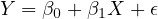
Endogeneity is a fundamental concept in econometrics that occurs when there is a correlation between an explanatory variable and the error term in a regression model. Consider a standard linear regression model:

In this model,  represents
the dependent variable,
represents
the dependent variable,  is an explanatory
variable, and
is an explanatory
variable, and  is the error term.
Endogeneity is present if
is the error term.
Endogeneity is present if  is endogenous,
which mathematically means that the covariance between
is endogenous,
which mathematically means that the covariance between  and
and  is not zero,
i.e.,
is not zero,
i.e., 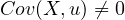 .
.
This correlation between the explanatory variable and the error term can arise from various sources such as omitted variables, measurement errors, or simultaneous causality. When endogeneity is present, it leads to biased and inconsistent estimators in regression analysis, posing significant challenges to drawing reliable conclusions about causal relationships.
1.2.3 Types and Examples of Endogeneity
Endogeneity can manifest in various forms in econometric analyses, each with its unique implications. This subsection discusses the main types of endogeneity.
Omitted Variable Bias
Omitted Variable Bias occurs when a relevant variable that influences the dependent variable and is correlated with the independent variable is left out of the analysis. This can lead to a misestimation of the effect of the included independent variables. OVB arises because the omitted variable may be capturing some effects that are wrongly attributed to the included variables.
Simultaneity
Simultaneity arises when there is bidirectional causality between the dependent and independent variables. A classic example is the relationship between economic growth and investment. Economic growth can lead to increased investment (as profits and capital become more available), while higher investment can in turn boost economic growth. This two-way causation presents a simultaneity issue in the model.
Measurement Error
Measurement Error occurs when the variables in a model are measured with error. This leads to inaccuracies in estimating the relationship between the variables. When key variables are not measured accurately, it undermines the reliability of the model’s estimations and can distort the actual impact of the variables.
1.2.4 Omitted Variable Bias
In econometric analyses, a common objective is to estimate the effect of certain
variables on outcomes of interest. Consider a study designed to estimate
the effect of class size ( ) on student test
scores (
) on student test
scores ( ). A significant
challenge in such analyses is the potential for omitted variable bias. This occurs
when a variable that influences the dependent variable is not included in the
model. For example, a student’s family background might affect both the class
size (
). A significant
challenge in such analyses is the potential for omitted variable bias. This occurs
when a variable that influences the dependent variable is not included in the
model. For example, a student’s family background might affect both the class
size ( ) and the test scores (
 ), but it may not be included in the
model.
), but it may not be included in the
model.
The omission of such a variable can have critical implications. In this example, both the class size and the family background could independently affect the test scores. Neglecting to account for family background can lead to a misestimation of the true effect of class size on test scores. This bias occurs because the omitted variable (family background) captures part of the effect that is incorrectly attributed to class size.
This situation gives rise to endogeneity due to the correlation between the omitted variable (family background) and the included variable (class size). In the regression model, this correlation manifests as a correlation between the error term and the class size, leading to biased estimates. The implications of such a bias are far-reaching. The estimated effect of class size on test scores might be either overestimated or underestimated. Policy decisions based on these biased estimates could end up being ineffective or even counterproductive.
To mitigate omitted variable bias, several strategies can be employed. If data on the omitted variable (like family background in our example) is available, it should be included in the model. Alternatively, the use of instrumental variables that are correlated with the class size but not with the error term can help. Additionally, conducting a sensitivity analysis to assess the robustness of the results to the inclusion of potentially omitted variables can provide insights into the reliability of the findings.
In econometric analyses, understanding the structure of the regression equation is crucial, especially when dealing with omitted variable bias. Consider the following scenario:
The true model, which represents the actual relationship including all relevant variables, is given by:
| (1) |

In Equation eq:true˙model,  is the dependent variable,
  and
and  are
independent variables, and
are
independent variables, and  is the error
term. The inclusion of
is the error
term. The inclusion of  is essential to
avoid bias in estimating the effect of
is essential to
avoid bias in estimating the effect of  on
on
 .
.
However, the estimated model often omits crucial variables due to various limitations like data availability. This model might be represented as:
| (2) |
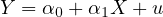
Omitting the variable  in
Equation eq:estimated˙model can lead to biased
estimates of
in
Equation eq:estimated˙model can lead to biased
estimates of  and
and  , particularly if
  is correlated with
  and has an
influence on
and has an
influence on  .
.
To understand the impact of  on the estimated model, consider expressing
 as a function of
  :
:
| (3) |

This expression captures the part of  that is and isn’t explained by
  .
.
When we substitute Equation eq:expression˙Z into the true model (Equation eq:true˙model), we obtain:
| (4) |

Equation eq:substituted˙model shows how the omitted variable  affects the
relationship between
affects the
relationship between  and
and  . The coefficient of
  now reflects a combination
of its direct effect on
now reflects a combination
of its direct effect on  and the indirect
effect via
and the indirect
effect via  .
.
The error term in the estimated model (Equation eq:estimated˙model) becomes:
| (5) |
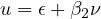
This error term is compounded by the omitted variable  ’s influence, captured by
 in Equation eq:error˙term. This leads to
endogeneity, characterized by a
non-zero covariance between
in Equation eq:error˙term. This leads to
endogeneity, characterized by a
non-zero covariance between  and
and  (
( ). Since
  contains
 and
and  is associated with
  (as
(as  is related to
  ), the error term
becomes correlated with
), the error term
becomes correlated with  . This correlation
results in biased and inconsistent
estimators.
. This correlation
results in biased and inconsistent
estimators.
The implication of this bias is significant, particularly in the interpretation of the
effect of  on
on  . The bias in the estimated coefficient
  in Equation
eq:estimated˙model means it fails to provide an accurate estimate of the true effect
in Equation
eq:estimated˙model means it fails to provide an accurate estimate of the true effect
 . This has serious implications in policy
analysis and prediction, where accurate
estimation of causal effects is critical.
. This has serious implications in policy
analysis and prediction, where accurate
estimation of causal effects is critical.
The bias in the estimated coefficient of  , denoted as
  , can be quantified
as:
, can be quantified
as:
| (6) |
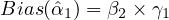
Equation eq:bias˙calculation shows that the omitted variable bias in the estimated
coefficient of  is the product of the true
effect of
is the product of the true
effect of  on
on  (
( )
and the
effect of
)
and the
effect of  on
on  (
( ). This leads to a misrepresentation of the effect of
  on
on
 , distorting the true understanding of the
relationship between these variables.
Such bias, if not addressed, can lead to misguided policy decisions. Accurate
estimation, therefore, requires addressing this bias, potentially through the inclusion
of
, distorting the true understanding of the
relationship between these variables.
Such bias, if not addressed, can lead to misguided policy decisions. Accurate
estimation, therefore, requires addressing this bias, potentially through the inclusion
of  in the model or via other statistical
methods like instrumental variable
analysis.
in the model or via other statistical
methods like instrumental variable
analysis.
Mitigating omitted variable bias (OVB) is crucial for the accuracy and reliability of econometric analyses. There are several strategies to address this issue:
Including the omitted variable, when observable and available, directly addresses OVB by incorporating the previously omitted variable into the regression model. This approach is only feasible when the omitted variable is measurable and data are available. Including the variable not only reduces bias but also improves the model’s explanatory power.
When the omitted variable cannot be directly measured or is unavailable, using proxy variables becomes an alternative strategy. A proxy variable, which is correlated with the omitted variable, can be used to represent it in the model. The proxy should ideally capture the core variation of the omitted variable. However, this method may not completely eliminate the bias, depending on how well the proxy represents the omitted variable.
The Instrumental Variables (IV) approach is another method used to mitigate OVB. In this approach, an instrumental variable is chosen that is uncorrelated with the error term but correlated with the endogenous explanatory variable (the variable affected by OVB). The IV approach helps in isolating the variation in the explanatory variable that is independent of the confounding effects caused by the omitted variable. The choice of a valid IV is crucial; it should influence the dependent variable only through its association with the endogenous explanatory variable. This method is commonly used in economics and social sciences, particularly when controlled experiments are not feasible.
Lastly, panel data and fixed effects models offer a solution when dealing with unobserved heterogeneity, where the omitted variable is constant over time but varies across entities, such as individuals or firms. These models help to control for time-invariant characteristics and isolate the effect of the variables of interest. Fixed effects models are especially useful for controlling for individual-specific traits that do not change over time and might be correlated with other explanatory variables.
Each of these methods has its strengths and limitations and must be carefully applied to ensure that the bias due to omitted variables is adequately addressed in econometric models.
1.2.5 Simultaneity in Economic Analysis
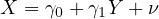
Understanding the relationship between economic growth and investment involves dealing with the issue of simultaneity. Economic growth can lead to more investment due to the availability of more profits and capital, while higher investment can, in turn, stimulate further economic growth. This mutual influence between economic growth and investment is a classic example of simultaneity, where each variable is endogenous, influencing and being influenced by the other. This simultaneous determination poses a significant challenge in identifying the causal direction and magnitude of impact between the two variables, making standard regression analysis inadequate.
Consider the investment function represented by:
| (7) |
In Equation eq:investment˙function,  represents investment,
  economic
growth, and
economic
growth, and  the random error term
capturing unobserved factors affecting
investment.
the random error term
capturing unobserved factors affecting
investment.
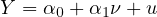
The economic growth function can be modeled as:
| (8) |
Here, Equation eq:growth˙function describes how economic growth  is influenced
by investment
is influenced
by investment  , with
  as the random error term for unobserved factors
affecting economic growth.
as the random error term for unobserved factors
affecting economic growth.
Substituting the economic growth function (Equation eq:growth˙function) into the investment function (Equation eq:investment˙function) gives us:
| (9) |

Equation eq:substituted˙function illustrates the endogenous determination of  and
and  , showcasing their interdependence.
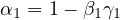
Simplifying this equation, we obtain:
| (10) |
where  ,
,  , and
, and 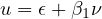 . In this model, the
error term
. In this model, the
error term  in Equation
eq:simplified˙function is correlated with
in Equation
eq:simplified˙function is correlated with  since
since  is
influenced by
is
influenced by  , and
, and  includes
  . This correlation implies endogeneity and
violates the Classical Linear Regression Model (CLRM) assumptions, leading to a
biased estimator for
. This correlation implies endogeneity and
violates the Classical Linear Regression Model (CLRM) assumptions, leading to a
biased estimator for  . The presence of
endogeneity complicates the interpretation
of regression results, particularly when assessing the effect of economic growth on
investment.
. The presence of
endogeneity complicates the interpretation
of regression results, particularly when assessing the effect of economic growth on
investment.
The implications of this endogeneity are significant for econometric analysis. The
bias in the estimator for  means that
conventional regression analysis will not
accurately capture the true effect of economic growth on investment. This
misrepresentation can lead to incorrect conclusions and potentially misguided policy
decisions.
means that
conventional regression analysis will not
accurately capture the true effect of economic growth on investment. This
misrepresentation can lead to incorrect conclusions and potentially misguided policy
decisions.
To address this issue, econometricians often resort to advanced techniques that can account for the simultaneity in the relationship between variables. One such approach is the use of structural models, where the simultaneous equations are estimated together, taking into account their interdependence. Another approach is using instrumental variables, where external variables that influence the endogenous explanatory variable but are not influenced by the error term in the equation are used to provide unbiased estimates.
The challenge, however, lies in correctly identifying and using these techniques, as they require strong assumptions and careful consideration of the underlying economic theory. Choosing an appropriate model or instrumental variable is crucial, as errors in these choices can lead to further biases and inaccuracies in the analysis.
In summary, simultaneity presents a complex challenge in econometric analysis, particularly in the study of relationships like that between economic growth and investment. Recognizing and addressing this simultaneity is key to uncovering the true nature of these economic relationships and providing reliable insights for policy-making and economic forecasting.
1.2.6 Measurement Error in Econometric Analysis
Understanding measurement error is crucial when estimating the effect of
variables in econometric models. Consider a study aiming to estimate the
effect of calorie intake ( ) on weight gain
(
) on weight gain
( ). Often, calorie intake is
self-reported or estimated, leading to measurement errors. This error is typically
not random and may be systematically biased due to underreporting or
misreporting.
). Often, calorie intake is
self-reported or estimated, leading to measurement errors. This error is typically
not random and may be systematically biased due to underreporting or
misreporting.
The nature of endogeneity in this context arises because the measured calorie
intake ( ) is
) is 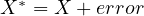 , where
  is the true calorie intake, and ‘error’
represents the measurement error. The correlation between the true calorie intake
(
is the true calorie intake, and ‘error’
represents the measurement error. The correlation between the true calorie intake
( ) and the measurement error causes
endogeneity. This correlation means that
the error in
) and the measurement error causes
endogeneity. This correlation means that
the error in  is related to
  itself, violating the Ordinary Least Squares
(OLS) assumption that the explanatory variables are uncorrelated with the error
term.
itself, violating the Ordinary Least Squares
(OLS) assumption that the explanatory variables are uncorrelated with the error
term.
The implications of this are significant. Estimates of the effect of calorie intake on
weight gain using the mismeasured variable  will be biased and inconsistent.
The direction of this bias depends on the nature of the measurement error, where
systematic underreporting or overreporting can lead to an underestimation or
overestimation of the true effect, respectively.
will be biased and inconsistent.
The direction of this bias depends on the nature of the measurement error, where
systematic underreporting or overreporting can lead to an underestimation or
overestimation of the true effect, respectively.
Mitigation strategies include using more accurate measurement methods for calorie intake, employing statistical techniques designed to address measurement error, such as Instrumental Variable (IV) methods, and conducting sensitivity analyses to understand the impact of potential measurement errors on the estimated effects.
The true model represents the actual relationship with the true, unobserved
variable  and is given by:
| (11) |
Here,  captures all other
unobserved factors affecting
captures all other
unobserved factors affecting  . However,
 is the
observed variable, which includes the true variable
is the
observed variable, which includes the true variable  and a measurement error
 :
:
| (12) |

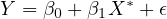
Substituting the observed variable  into the true model gives us the substituted
model:
into the true model gives us the substituted
model:
| (13) |

The new error term now includes the measurement error. This leads to an altered error term in the regression with the observed variable:
| (14) |
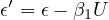
Since  includes
  , and
, and  is part of
  ,
,  is correlated with
 , violating the OLS assumption that the
explanatory variable should
be uncorrelated with the error term. This correlation leads to biased and
inconsistent estimates of
, violating the OLS assumption that the
explanatory variable should
be uncorrelated with the error term. This correlation leads to biased and
inconsistent estimates of  , with the
direction and magnitude of bias dependent
on the nature of the measurement error and its relationship with the true
variable.
, with the
direction and magnitude of bias dependent
on the nature of the measurement error and its relationship with the true
variable.
The presence of measurement error, particularly in a key explanatory variable like
calorie intake, can significantly distort the findings of a regression analysis. As illustrated
in the substituted model (Equation eq:substituted˙model˙measurement˙error), the
inclusion of the measurement error in the error term (Equation eq:new˙error˙term)
complicates the estimation process. The correlation of  with
with  , as per
Equation eq:new˙error˙term, indicates that the standard Ordinary Least
Squares (OLS) estimator will be biased and inconsistent, leading to unreliable
estimates.
, as per
Equation eq:new˙error˙term, indicates that the standard Ordinary Least
Squares (OLS) estimator will be biased and inconsistent, leading to unreliable
estimates.
This bias in the estimator  signifies that the estimated effect of calorie intake
on weight gain, when relying on the mismeasured variable
signifies that the estimated effect of calorie intake
on weight gain, when relying on the mismeasured variable  , will not accurately
reflect the true effect. The direction and magnitude of this bias are contingent upon
the nature and extent of the measurement error. For instance, if the error is
predominantly due to systematic underreporting, the estimated effect may be
understated. Conversely, systematic overreporting could result in an overstated
effect.
, will not accurately
reflect the true effect. The direction and magnitude of this bias are contingent upon
the nature and extent of the measurement error. For instance, if the error is
predominantly due to systematic underreporting, the estimated effect may be
understated. Conversely, systematic overreporting could result in an overstated
effect.
To mitigate the impact of measurement error, researchers must consider several strategies. Firstly, adopting more accurate methods to measure the key variables can significantly reduce the likelihood of measurement error. When direct measurement is challenging, using proxy variables that closely represent the true variable can be an alternative, though this approach may still retain some level of bias.
Moreover, the use of advanced econometric techniques, such as Instrumental Variable (IV) methods, provides a robust way to address endogeneity arising from measurement error. These methods rely on finding an instrument that is correlated with the mismeasured variable but uncorrelated with the error term, allowing for a more reliable estimation of the causal effect. However, finding a valid instrument can be challenging and requires careful consideration and validation.
Lastly, conducting sensitivity analyses is crucial to assess the robustness of the results to potential measurement errors. These analyses can help in understanding the extent to which measurement error might be influencing the estimated relationships and provide insights into the reliability of the conclusions drawn from the analysis.
In conclusion, measurement error poses a significant challenge in econometric modeling, particularly when key variables are prone to inaccuracies in measurement. Recognizing and addressing this issue is essential for ensuring the validity and reliability of econometric findings, especially in fields where accurate measurements are difficult to obtain.
1.2.7 Understanding Selection Bias
Selection bias is a critical issue in statistical analysis and econometrics, occurring when the samples in the data are not randomly selected. This bias arises in situations where the mechanism of data collection or the nature of the process being studied leads to a non-random subset of observations being analyzed. It is common in observational studies, especially in the social sciences and economics, where randomization is not always possible.
The presence of selection bias violates the assumptions of the Classical Linear Regression Model (CLRM), particularly the assumption that the error term is uncorrelated with the explanatory variables. This violation occurs because the non-random sample selection introduces a systematic relationship between the predictors and the error term, potentially leading to biased and misleading results in regression analysis. As a consequence, the estimates obtained may not accurately represent the true relationship in the population, which can lead to incorrect inferences and policy decisions.
Examples and common sources of selection bias include studies where participants self-select into a group or where data is only available for a specific subset of the population. For instance, in health studies examining the effect of diet on health, there may be an upward bias in the estimated diet effect if health-conscious individuals are more likely to participate. Similarly, in educational research, studying the impact of private schooling on achievement might lead to an overestimation of private schooling benefits if there is a selection of students based on parental dedication. Another example is in economic studies comparing earnings by education level, where college attendees are non-random and influenced by various factors, resulting in earnings comparisons being biased by unobserved factors like ability or background.
Mitigating selection bias involves employing techniques such as propensity score matching, instrumental variable analysis, or Heckman correction models. These methods aim to account for the non-random selection process and adjust the analysis accordingly. Additionally, ensuring a randomized selection process, if feasible, or accounting for the selection mechanism in the analysis, can help in reducing the impact of selection bias.
In summary, selection bias presents a significant challenge in statistical analysis, particularly in fields where controlled experiments are not feasible. Recognizing, understanding, and addressing this bias are essential steps in conducting robust and reliable econometric research.
1.2.8 Concluding Remarks: Navigating Endogeneity and Selection Bias
Navigating the complexities of endogeneity and selection bias is crucial in econometric models to ensure accurate causal inference and reliable research results. Endogeneity, a pervasive issue in econometrics, leads to biased and inconsistent estimators. It primarily arises from three sources: omitted variable bias, simultaneity, and measurement error. Each of these sources contributes to the distortion of the estimations in its way, making it imperative to understand and address endogeneity comprehensively.
In parallel, selection bias presents a significant challenge in research, particularly when samples are non-randomly selected. This bias is common in various research contexts, ranging from health studies to education and economic research. It leads to misleading results that may not accurately reflect the true dynamics of the population or process under study. To mitigate the effects of selection bias, researchers must remain vigilant in their research design and employ appropriate techniques. Strategies such as propensity score matching and Heckman correction are commonly used to adjust for selection bias, especially in observational studies where randomization is not feasible.
Mitigation strategies for endogeneity include the use of instrumental variables, fixed effects models, and, where possible, randomized controlled trials. These methods aim to isolate the causal relationships and minimize the influence of confounding factors. Similarly, for addressing selection bias, techniques that account for the non-random selection process are essential. The overall significance of effectively dealing with these challenges cannot be overstated. Recognizing and appropriately addressing endogeneity and selection bias are fundamental to conducting robust and valid econometric analysis, leading to more accurate interpretations and sound policy implications.
1.3 Multicollinearity and Causality Identification
1.3.1 Introduction
In this section of the textbook, we delve into the intricate concepts of multicollinearity and causality identification, which are cornerstone topics in the field of econometrics. These concepts are not only foundational in understanding the dynamics of economic data but also crucial in crafting rigorous econometric models and making informed policy decisions.
Multicollinearity refers to a scenario within regression analysis where two or more independent variables exhibit a high degree of correlation. This collinearity complicates the model estimation process, as it becomes challenging to distinguish the individual effects of correlated predictors on the dependent variable. The presence of multicollinearity can severely impact the precision of the estimated coefficients, leading to unstable and unreliable statistical inferences. It’s a phenomenon that, while not affecting the model’s ability to fit the data, can significantly undermine our confidence in identifying which variables truly influence the outcome.
Addressing multicollinearity involves a careful examination of the variables within the model and, often, the application of techniques such as variable selection or transformation, and in some cases, the adoption of more sophisticated approaches like ridge regression. These strategies aim to mitigate the adverse effects of multicollinearity, thereby enhancing the model’s interpretability and the reliability of its conclusions.
On the other hand, causality identification moves beyond the mere recognition of patterns or correlations within data to ascertain whether and how one variable causally influences another. This exploration is pivotal in economics, where understanding the causal mechanisms behind observed relationships is essential for effective policy-making. Identifying causality allows economists to infer more than just associations; it enables them to uncover the underlying processes that drive economic phenomena.
However, multicollinearity poses challenges in causality identification, as it can obscure the true relationships between variables. When predictors are highly correlated, disentangling their individual causal effects becomes increasingly difficult. This complexity necessitates the use of advanced econometric techniques, such as instrumental variable (IV) methods, difference-in-differences (DiD) analysis, or regression discontinuity design (RDD), each of which offers a pathway to uncover causal relationships under specific conditions.
In summary, both multicollinearity and causality identification are critical in the econometric analysis, providing the tools and insights necessary to understand and model the economic world accurately. Through real-world examples and case studies, this section aims to equip you with a comprehensive understanding of these concepts, emphasizing their importance in econometric modeling and the formulation of economic policy. As we explore these topics, you will gain a clearer perspective on the role and significance of multicollinearity and causality in econometric research, enabling you to apply these concepts effectively in your analytical endeavors.
1.3.2 Multicollinearity
Multicollinearity represents a significant concern in regression analysis, characterized by a scenario where two or more predictors exhibit a high degree of correlation. This condition complicates the estimation process, as it challenges the assumption that independent variables should, ideally, be independent of each other. In the context of multicollinearity, this independence is compromised, leading to potential issues in interpreting the regression results.
There are two primary forms of multicollinearity: perfect and imperfect. Perfect multicollinearity occurs when one predictor variable can be precisely expressed as a linear combination of others. This situation typically mandates the removal or transformation of the involved variables to proceed with the analysis. On the other hand, imperfect multicollinearity, characterized by a high but not perfect correlation among predictors, is more common and subtly undermines the reliability of the regression coefficients.
The consequences of multicollinearity are manifold and primarily manifest in the inflation of the standard errors of regression coefficients. This inflation can significantly reduce the statistical power of the analysis, thereby making it more challenging to identify the true effect of each independent variable. High standard errors lead to wider confidence intervals for coefficients, which in turn decreases the likelihood of deeming them statistically significant, even if they genuinely have an impact on the dependent variable.
Understanding and addressing multicollinearity is crucial for econometricians. Techniques such as variance inflation factor (VIF) analysis can diagnose the severity of multicollinearity, guiding researchers in deciding whether corrective measures are necessary. Depending on the situation, solutions may involve dropping one or more of the correlated variables, combining them into a single predictor, or applying regularization methods like ridge regression that can handle multicollinearity effectively.
In sum, recognizing and mitigating the effects of multicollinearity is imperative for ensuring the accuracy and interpretability of regression analyses. By carefully examining the relationships among predictors and employing appropriate statistical techniques, econometricians can overcome the challenges posed by multicollinearity, thereby enhancing the robustness of their findings.
1.3.3 Example 1: Multicollinearity in Housing Market Analysis
In the context of a regression model analyzing the housing market, consider the following basic equation:
| (15) |

where  represents the house
price (dependent variable),
represents the house
price (dependent variable),  denotes the
size
of the house (e.g., in square feet), and
denotes the
size
of the house (e.g., in square feet), and  indicates the number of rooms in the
house.
indicates the number of rooms in the
house.
This example illustrates the concept of multicollinearity, a scenario where the
independent variables  (size of the house)
and
(size of the house)
and  (number of rooms) are
likely to be highly correlated. Such a high correlation between these variables
suggests that they are not truly independent, which is a hallmark of multicollinearity.
The presence of multicollinearity can significantly increase the variance of the
coefficient estimates, making it difficult to determine the individual impact of each
independent variable on the dependent variable. Consequently, this challenges the
reliability of the regression model and complicates the interpretation of its
results.
(number of rooms) are
likely to be highly correlated. Such a high correlation between these variables
suggests that they are not truly independent, which is a hallmark of multicollinearity.
The presence of multicollinearity can significantly increase the variance of the
coefficient estimates, making it difficult to determine the individual impact of each
independent variable on the dependent variable. Consequently, this challenges the
reliability of the regression model and complicates the interpretation of its
results.
To address multicollinearity, one might consider revising the model to mitigate its effects, such as by removing one of the correlated variables or by combining them into a single composite variable. Alternatively, employing advanced techniques like Ridge Regression could help manage the issue by introducing a penalty term that reduces the magnitude of the coefficients, thereby diminishing the problem of multicollinearity.
This example underscores the importance of recognizing and addressing multicollinearity in econometric modeling, particularly in studies involving inherently related variables, such as those found in housing market analysis. By taking steps to mitigate multicollinearity, researchers and analysts can enhance the accuracy and interpretability of their models, leading to more reliable and insightful conclusions.
1.3.4 Example 2: Multicollinearity in Economic Growth Analysis
In the realm of econometric modeling focused on understanding the factors that influence a country’s annual GDP growth, consider the following model:
| (16) |

where  signifies the annual
GDP growth,
signifies the annual
GDP growth,  represents the country’s
expenditure on education, and
represents the country’s
expenditure on education, and  denotes the
country’s literacy rate.
denotes the
country’s literacy rate.
This model presents a classic scenario of multicollinearity, particularly due to the
likely high correlation between education expenditure ( ) and literacy rate
(
) and literacy rate
( ). The interconnectedness of these
variables challenges their assumed
independence in predicting GDP growth, illustrating the phenomenon of
multicollinearity. The presence of such multicollinearity can complicate the accurate
assessment of the individual impacts of education expenditure and literacy rate on
GDP growth. Consequently, the reliability of coefficient interpretations is
undermined, which can lead to misguided policy recommendations if not addressed
properly.
). The interconnectedness of these
variables challenges their assumed
independence in predicting GDP growth, illustrating the phenomenon of
multicollinearity. The presence of such multicollinearity can complicate the accurate
assessment of the individual impacts of education expenditure and literacy rate on
GDP growth. Consequently, the reliability of coefficient interpretations is
undermined, which can lead to misguided policy recommendations if not addressed
properly.
To mitigate the effects of multicollinearity in this context, researchers might employ advanced statistical techniques such as principal component analysis (PCA) to create new independent variables that capture the essence of both education expenditure and literacy rate without the high correlation. Alternatively, re-specifying the model or incorporating additional data could provide clarity on the distinct effects of these variables on GDP growth.
Such strategies are vital in ensuring the robustness of econometric analyses, especially when exploring complex relationships like those between education, literacy, and economic growth. By addressing multicollinearity effectively, the model’s predictive power and the validity of its policy implications can be significantly enhanced.
1.3.5 Detecting Multicollinearity
Detecting multicollinearity is a pivotal step in the regression analysis process, aimed at ensuring the accuracy and reliability of model coefficients. Multicollinearity occurs when independent variables within a regression model are highly correlated, potentially distorting the estimation of model coefficients and weakening the statistical power of the analysis.
One primary tool for identifying multicollinearity is the Variance
Inflation
Factor (VIF). The VIF quantifies how much the variance of a regression coefficient
is increased due to multicollinearity, comparing it with the scenario where the
predictor variables are completely linearly independent. Mathematically, for a given
predictor  , the VIF is defined as:
| (17) |
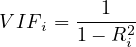
where  is the coefficient of determination of a regression of
  on all the
other predictors. A VIF value exceeding 10 often signals the presence of significant
multicollinearity, necessitating corrective measures.
on all the
other predictors. A VIF value exceeding 10 often signals the presence of significant
multicollinearity, necessitating corrective measures.
Another important metric is tolerance, which is simply the inverse of VIF. Tolerance measures the proportion of variance in a predictor not explained by other predictors, with lower values indicating higher multicollinearity:
| (18) |
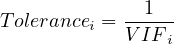
Both high VIF values and low tolerance levels serve as indicators that predictor variables are highly correlated. This correlation can obscure the individual contributions of predictors to the dependent variable, complicating the interpretation of the model.
To effectively manage multicollinearity, it is advisable to regularly assess these metrics, especially in models with a large number of predictors. Strategies for addressing detected multicollinearity may include revising the model by removing or combining correlated variables or applying dimensionality reduction techniques such as principal component analysis (PCA). These actions aim to refine the model for enhanced interpretability and validity.
In summary, vigilant detection and management of multicollinearity are essential for conducting robust regression analysis. By applying these principles and leveraging statistical tools like VIF and tolerance, researchers can mitigate the adverse effects of multicollinearity and draw more reliable conclusions from their econometric models.
1.3.6 Addressing Multicollinearity
Addressing multicollinearity is a crucial aspect of refining regression models to enhance their interpretability and the accuracy of the estimated coefficients. Multicollinearity arises when independent variables in a regression model are highly correlated, which can obscure the distinct impact of each variable. The primary goal in addressing multicollinearity is to reduce the correlation among independent variables without significantly compromising the information they provide.
One approach to mitigate multicollinearity involves data transformation and variable selection. Techniques such as logarithmic transformation or the creation of interaction terms can sometimes alleviate the issues caused by multicollinearity. Additionally, careful selection of variables, particularly avoiding those that are functionally related, can significantly reduce multicollinearity in the model. For instance, if two variables are highly correlated, one may consider excluding one from the model or combining them into a new composite variable that captures their shared information.
Ridge Regression offers another solution to multicollinearity. This method extends linear regression by introducing a regularization term to the loss function, which penalizes large coefficients. This regularization can effectively diminish the impact of multicollinearity, particularly in models with a large number of predictors. The regularization term is controlled by a parameter that determines the extent to which coefficients are penalized, allowing for a balance between fitting the model accurately and maintaining reasonable coefficient sizes.
When addressing multicollinearity, several practical considerations must be taken into account. Each method to reduce multicollinearity comes with its trade-offs and should be selected based on the specific context of the study and the characteristics of the data. It is vital to assess the impact of these techniques on the model’s interpretation, ensuring that any adjustments do not compromise the theoretical integrity or practical relevance of the analysis.
Adopting an iterative approach to model building is essential. After applying techniques to reduce multicollinearity, it is crucial to reassess the model to determine the effectiveness of these adjustments. Diagnostic tools, such as the Variance Inflation Factor (VIF), can be invaluable in this process, providing a quantifiable measure of multicollinearity for each independent variable. Continuously monitoring and adjusting the model as needed helps ensure that the final model is both statistically robust and theoretically sound.
1.3.7 Multicollinearity and Causality Identification
The interplay between multicollinearity and causality identification presents a nuanced challenge in econometric analysis, particularly when attempting to discern the direct influence of individual variables within a regression model. Multicollinearity, characterized by a high correlation among independent variables, complicates the isolation of single variable effects, thereby muddying the waters of causal inference. This becomes acutely problematic in policy analysis, where a precise understanding of each variable’s unique impact is paramount for informed decision-making.
Multicollinearity’s tendency to mask the true causal relationships within data can lead researchers to draw incorrect conclusions about the determinants of observed outcomes. For instance, when two or more predictors are closely interlinked, distinguishing between their individual contributions to the dependent variable becomes fraught with difficulty, potentially resulting in the misattribution of effects.
Moreover, the presence of multicollinearity can induce specification errors in model design, such as omitted variable bias, where the exclusion of relevant variables leads to a skewed representation of the causal dynamics at play. These errors not only distort the perceived relationships among the variables but can also falsely suggest causality where none exists or obscure genuine causal links.
The application of instrumental variables (IV) for causal inference further illustrates the complexities introduced by multicollinearity. Ideally, an instrumental variable should be strongly correlated with the endogenous explanatory variable it is meant to replace but uncorrelated with the error term. However, multicollinearity among explanatory variables complicates the identification of suitable instruments, as it can be challenging to find instruments that uniquely correspond to one of the collinear variables without influencing others.
Addressing these challenges necessitates a careful and deliberate approach to model selection and testing. By actively seeking to mitigate the effects of multicollinearity—whether through variable selection, data transformation, or the application of specialized econometric techniques—researchers can enhance the clarity and reliability of causal inference. Ultimately, the rigorous examination of multicollinearity and its implications for causality is indispensable for advancing robust econometric analyses that can underpin sound empirical research and policy formulation.
1.3.8 Conclusion
In wrapping up our discussion on multicollinearity and causality identification, we’ve traversed the intricate landscape of these pivotal concepts in econometric analysis. The exploration has underscored the significance of understanding and addressing multicollinearity, a factor that, though sometimes neglected, is crucial for the accuracy and interpretability of regression models. Furthermore, the delineation between correlation and causation emerges as a cornerstone in empirical research, serving as a beacon for informed policy-making and decision processes.
Addressing Multicollinearity: Our journey included a review of methodologies to detect and ameliorate the effects of multicollinearity, such as employing data transformation, judicious variable selection, and the application of ridge regression. These strategies are instrumental in refining econometric models to yield more reliable and decipherable outcomes.
Emphasizing Causality: The dialogue accentuated the importance of techniques like Randomized Controlled Trials (RCTs), Instrumental Variables (IV), Difference-in-Differences (DiD), and Regression Discontinuity Design (RDD) in the establishment of causal relationships. Mastery and appropriate application of these methods fortify the robustness and significance of econometric analyses, paving the way for compelling empirical evidence.
Integrating Concepts in Research: The intricate relationship between multicollinearity and causality identification highlights the imperative for meticulous and discerning econometric analysis. For those embarking on the path of economics and research, the adept navigation through these concepts is paramount in conducting meaningful empirical inquiries.
Final Thoughts: I urge you to integrate these insights into your research endeavors thoughtfully. It is essential to remain vigilant of the assumptions and limitations inherent in your models, ensuring that your work not only adheres to rigorous statistical standards but also contributes valuable insights to the field of economics. As we continue to advance in our understanding and application of these principles, we pave the way for more nuanced and impactful econometric research.